
On the global dynamics of the Newell–Whitehead system
- DOI
- 10.1080/14029251.2019.1640466How to use a DOI?
- Keywords
- Global dynamics; Poincaré compactification; Newell–Whitehead system; invariant algebraic curve; invariant
- Abstract
In this paper by using the Poincaré compactification in ℝ3 we make a global analysis of the model x′ = z, y′ = b(x−dy), z′ = x(x2 −1)+y+cz with b ∈ ℝ and c, d ∈ ℝ+, here known as the three-dimensional Newell–Whitehead system. We give the complete description of its dynamics on the sphere at infinity. For some values of the parameters this system has invariant algebraic surfaces and for these values we provide the dynamics of the system restricted to these surfaces and its global phase portrait in the Poincaré ball. We also include the description of the α-limit and ω-limit set of its orbits in the Poincaré ball including its boundary, that is, in the compactification of ℝ3 with the sphere at the infinity. We recall that the restricted systems are not analytic and so in this paper we overcome this difficulty by using the blow-up technique.
- Copyright
- © 2019 The Authors. Published by Atlantis and Taylor & Francis
- Open Access
- This is an open access article distributed under the CC BY-NC 4.0 license (http://creativecommons.org/licenses/by-nc/4.0/).
1. Introduction and statement of the results
The FitzHugh-Nagumo system is written as
These equations were introduced by FitzHugh [5] and Nagumo [9]. In [5], the author simplified the four dimensional Hodgkin-Huxley system into a planar system (called Bonhoeffer-Van der Por system) and he also considered the excitable and oscillatory behavior of the Bonhoeffer-Van der Por system and showed the underlying relationship between the Bonhoeffer-Van der Por system and the BVP system and Hodgkin-Huxley system. By the method used in [5] and the Kirchhoff’s law, the authors in [9] considered the propagation of the excitation along the nerve axon into the Hodgkin-Huxley system, and the Hodgkin-Huxley system becomes the FitzHugh-Nagumo partial differential equation. This system has been intensively studied in the literature mainly due to its simplicity for describing the excitation of neural membranes and the propagation of nerve impulses along an axon. This has caused the attention of many authors that studied, among others aspects of the system, the existence, uniqueness and stability of its traveling wave solutions (see [2,3,6,7,9–11]). If we assume the existence of a traveling wave solution for the FitzHugh-Nagumo partial differential equation that is a bounded solution (u(x,t),v(x,t)) with x, t ∈ ℝ satisfying (u(x,t),v(x,t)) = (u(x+ct),v(x+ct)) being c > 0 the constant denoting the wave speed and we substitute it into the FitzHugh-Nagumo partial differential equation, we get the following ordinary differential equation
The integrability of system (1.1) has been studied in [12] where the authors give the description of all the invariant algebraic surfaces of the system. Let U be an open subset of ℝ3. A first integral H : U → ℝ of system (1.1) is a function which is constant on the trajectories of the system. A function I(x,y,z,t) is an invariant of system (1.1) if dI/dt = 0 on the trajectories of the system, that is, an invariant is a first integral which depends on time. The following proposition proved in [12] summarizes the results on the integrability and on the existence of invariants for system (1.1).
Proposition 1.1.
The following holds for system (1.1).
- (i)
if bd = −c,
- (ii)
if
Proposition 1.1 will be used in the following sections for studying the global dynamics behavior of system (1.1) having an invariant. As any polynomial differential system, system (1.1) can be extended to an analytic system on a closed ball of radius one, whose interior is diffeomorphic to ℝ3 and its invariant boundary, a two-dimensional sphere 𝕊2 plays the role of infinity. This ball will be denoted by B and called the Poincaré ball, due to the fact that the technique for doing so is the Poincaré compactification, which is well established (see, for instance [4]). Two polynomial vector fields are said to be topologically equivalent if there exists a homeomorphism on the closed Poincaré ball preserving the infinity (that is the boundary of the Poincaré ball) carrying orbits of the flow induced on the Poincaré ball by the first vector field into orbits of the flow induced in the Poincaré ball by the second vector field.
By using this compactification technique we can describe the dynamics of system (1.1) at infinity. This is the first main result of the paper.
Theorem 1.1.
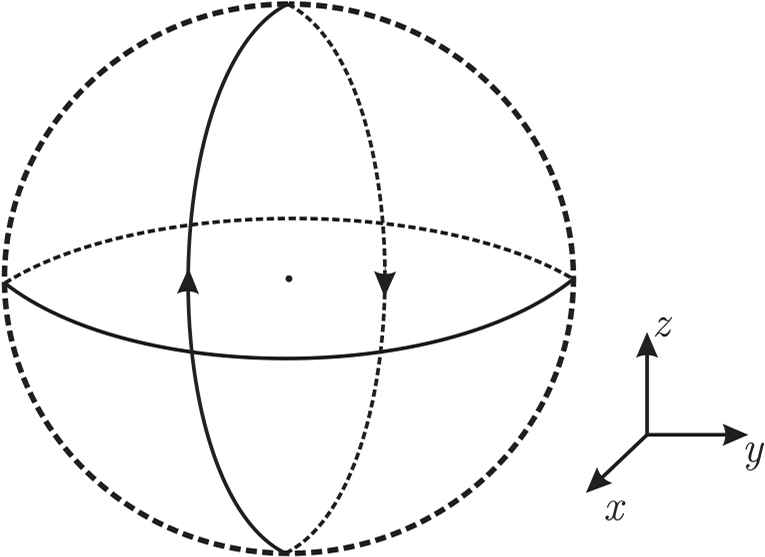
For all values of the parameters b ∈ ℝ and c, d ∈ ℝ+, the phase portrait of system (1.1) on the Poincaré sphere is topologically equivalent to the one shown in Figure 1.
Note that the dynamics at infinity do not depend on the parameter values. The proof of Theorem 1.1 is given in Section 3 by means of the Poincaré compactification technique.
Now we continue the study of the dynamics of system (1.1) for the values of the parameters in Proposition 1.1. We provide the description of the global dynamics of the this polynomial differential system not only on ℝ3 but also in its compactification for some values of the parameters. In particular, we will study the dynamics on the whole ℝ3 including the behavior on the sphere at infinity, that is, on the Poincaré ball and we describe the α-limit sets and the ω-limit sets of all bounded orbits of the system (1.1) for some values of the parameters.
Theorem 1.2.
The global phase portraits of system (1.1) on the Poincaré ball for the values of the parameters in Proposition 1.1 are topologically equivalent to the ones described in Figure 2.
The proof of Theorem 1.2 is given in Section 4.
2. Preliminaries
First we recall a well-known result that was proved in [8].
Lemma 2.1.
Let F(x,y,z) = 0 be a degree m algebraic surface of ℝ3. The extension of this surface to the boundary of the Poincaré ball is contained in the curve defined by
Lemma 2.2.
If ϕ (t) = (x(t),y(t),v(t)), t ∈ ℝ is a bounded trajectory of system (1.1) satisfying the assumptions of statements (i) and (ii) in Proposition 1.1 with invariants
Proof.
Let q1 ∈ ω(ϕ). Thus there exists tn → ∞ such that ϕ (tn) → q1. Thus
Thus K = 0 and then
Assume now that q2 ∈ α(ϕ). Then there exists tn → −∞ such that ϕ (tn) → q2. Hence
Now we study the limit cycles of this system under the assumptions of Proposition 1.1.
Lemma 2.3.
Under the assumptions of Proposition 1.1, system (1.1) has no limit cycles.
Proof.
Since the cofactors of the invariant algebraic surfaces are constant, if the limit cycle exists, it must be located on the invariant surface. Taking into account that the divergence of system (1.1) is c − bd and that on the values of the parameters provided by Proposition 1.1 the divergence is different from zero we conclude that such limit cycle cannot exist.
Now we study the finite singular points under the assumptions of Proposition 1.1. We recall that the stability index of a hyperbolic point is the number of eigenvalues with negative real part.
Lemma 2.4.
The following holds for system (1.1) under the assumptions (i) or (ii) in Proposition 1.1.
- (a)
If d ∈ (0,1] the origin is the unique singular point;
- (b)
If d > 1 besides the origin there are the two additional singular points
- (c)
The Jacobian matrix at the origin of system (1.1) under the assumptions (i) has eigenvalues 2c/3 and
- (d)
The Jacobian matrix at the two points S± of system (1.1) under the assumptions (i) has the eigenvalues 4c/3 and
Proof.
The proof of the lemma follows by direct calculations.
3. Proof of Theorem 1.1
For studying the infinity of the Poincaré ball B we analyze the flow at infinity for the local charts U1, U2 and U3. In the next subsecti ons we study the Poincaré compactification of system (1.1) in the local charts U1, U2, U3 and V1, V2, V3.
3.1. Study of the infinite in the local charts U1 and V1
The Poincaré compactification of system (1.1) in the local chart U1 is given by
For z3 = 0 (which corresponds to the points on the sphere 𝕊2 at infinity) system (3.1) becomes
This system has no equilibria. The solution is given by parallel straight lines to the z2-axis. The flow on the local chart V1 is the same than the flow of U1, because the compactified vector field in V1 coincides with the vector field in U1 multiplied by (−1)3−1 = 1.
3.2. Study of the infinite in the local charts U2 and V2
The expression of the Poincaré compactification in the local chart U2 of system (1.1) writes as
System (3.3) restricted to z3 = 0 becomes
System (3.4) has the plane z1 = 0 of equilibria. Considering the invariance of the z1z2-plane under the flow of (3.3) we can completely describe the dynamics on the sphere at infinity, which is shown in Figure 1. Note that this system for z1 ≠ 0 is equivalent to system (3.2) and the plane z1 = 0 is a plane of equilibria. Again the flow on the local chart V2 is the same as the flow on the local chart U2.
3.3. Study of the infinite in the local charts U3 and V3
The expression of the Poincaré compactification of system (1.1) in the local chart U3 is given by
Observe that system (3.5) restricted to the invariant z1z2-plane reduces to
The solution of this system corresponds to the dynamics of system (3.3) in the local chart U3. Note that z1 = 0 is a line of equilibria. For z1 ≠ 0 the system is equivalent to
Proof of Theorem 1.1.
Considering the analysis made in the previous subsections and gluing the flow in the three studied charts, we have a global picture of the dynamical behavior of system (1.1) at infinity given in Figure 1. The system has one closed curve of equilibria which is x = 0, y2 +z2 = 1 and there are no equilibrium points in the sphere. We observe that the description of the complete phase portrait of system (1.1) on the sphere at infinity (the Poincaré ball) was possible because of the invariance of these sets under the flow of the compactified system. This proves Theorem 1.1. We remark that the behavior of the flow at infinity does not depend on the parameters of the system.
4. Proof of Theorem 1.2
In this section we prove Theorem 1.2. We consider the invariants given in Proposition 1.1 and how the surfaces end in the Poincaré sphere at infinity.
4.1. Case bd = −c, c ≠ 0, b = 2 27 c 3 − 1 3 c 0 < c < 3 2
In this case
According to Lemma 2.1 the boundary of this surface on the sphere 𝕊2 of the infinity is given by the system
Now we study the dynamics of equation (1.1) on this invariant surface when x ≠ 0. If x ≠ 0 the restriction of system (1.1) to the invariant surface is given by
This system has, among the origin, two finite singular points with x ≠ 0 which are
The eigenvalues of the Jacobian matrix at these points are
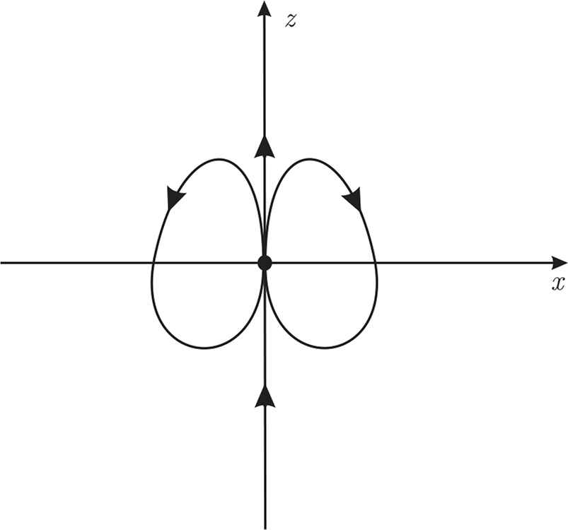
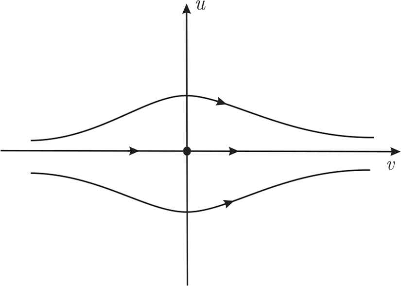
Local phase portrait of system (4.1) at the origin.
Now we study the dynamics at infinity by means of the Poincaré compactification for system (4.1). On the local chart U1 we get the system
Note that this system has no singular points on v = 0 and so there are no singular points in the local chart U1. On the local chart U2 we get
Note that the origin of the local chart U2 is a singular point which is degenerate. Doing again a blow-up we get that its local phase portrait is topologically equivalent to a node.
Taking into account the analysis on the surface together with the infinity and Lemma 2.3 we get the global phase portrait of system (4.1) on the Poincaré disc shown in Figure 4.
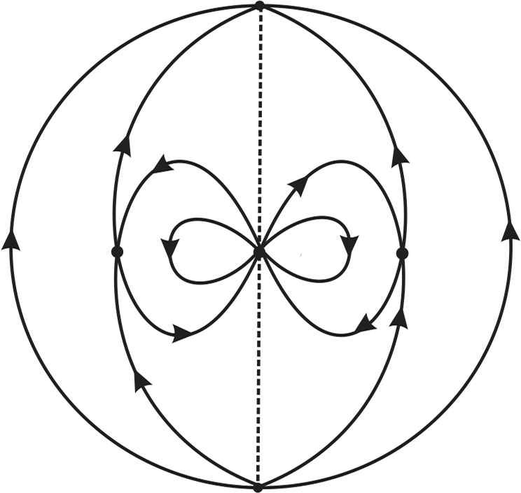
Phase portrait of system (4.1) on the Poincaré disc.
To obtain the global phase portrait on the Poincaré sphere given in Figure 4 we use the information above (on the boundary at infinity and on the surface F2 = 0) together with Lemma 2.4 which guarantees that the origin is in this case a global repeller.
According to Lemma 2.2 for any trajectory not contained in the invariant surface we have that the ω-limit is contained in {F2 = 0} and the α-limit is contained in 𝕊2 (that is, it is the point (0, ±1,0)).
The complete phase portrait given in Figure 2 can be obtained with the union of the Figure 4 with the infinity sphere.
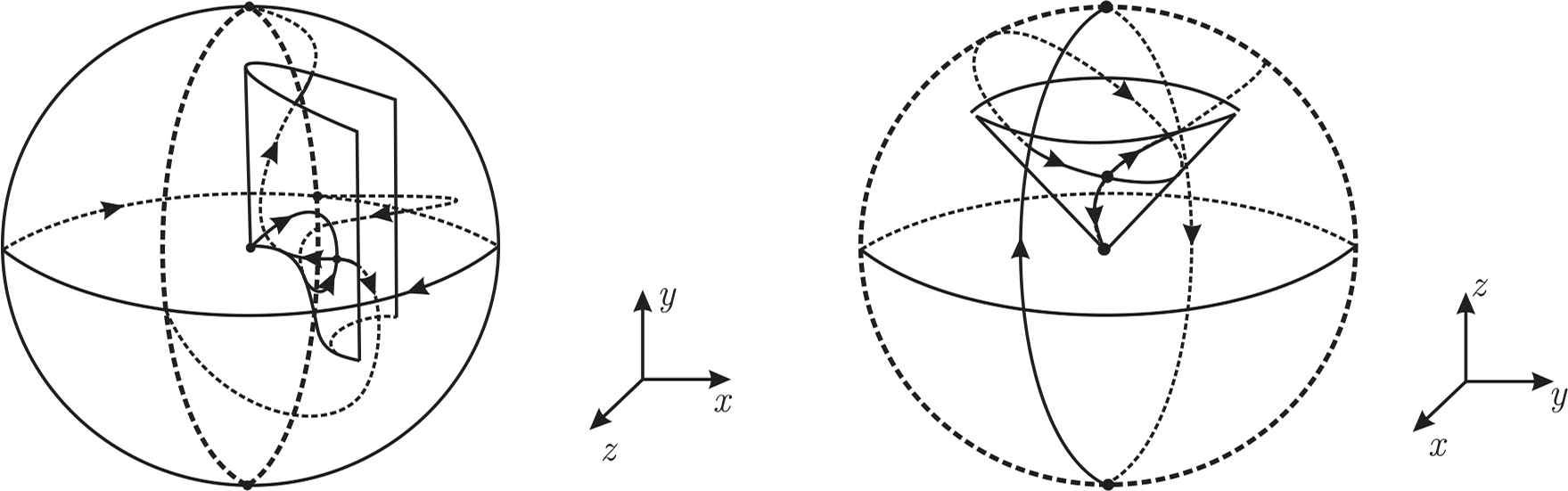
Global phase portraits of system (1.1) under the assumptions of Proposition 1.1(i) on the left and under the assumptions of Proposition 1.1(ii) on the right.
4.2. Case b d = − 2 3 c b = 2 27 c 3 − c 3 0 < c < 3 2
The invariant algebraic surface is
According to Lemma 2.1 the boundary of this surface on the sphere 𝕊2 of the infinity is given by
Now we will study the dynamics of system (1.1) on the surface F3 = 0 projected onto the (x,y)-plane. The surface F3 = 0 yields
The projected systems taking z± is given by
Among the origin, this system has the singular points
The eigenvalues of R+ for the restriction on z+ (respectively of R− for the restriction on z−) are
Note that systems (4.2) are not analytic at the origin. In order to study its local behavior at the origin we analyze the original system (1.1). In view of Lemma 2.4, taking into account that
Now we consider the dynamics at the infinity. Note that the topological structure of both systems in (4.2) are the same and so we will only work with the projection on z+. Taking the Poincaré transformation x = 1/v, y = u/v with the scaling dτ = vdt we get the system
Note that the origin is a singular point which is a stable node. On the other hand, taking the Poincaré transformation x = u/v, y = 1/v with the time scaling dτ = vdt, the system becomes
The origin is a degenerate singular point. Doing a blow-up we conclude that its local phase portrait is topologically equivalent to the one of Figure 5.
Local phase portrait of the origin of system (4.3).
Combining the study on the finite plane and at infinity together with Lemma 2.3 we get that the global phase portrait of system (1.1) on F3 = 0 is the one given in Figure 6.
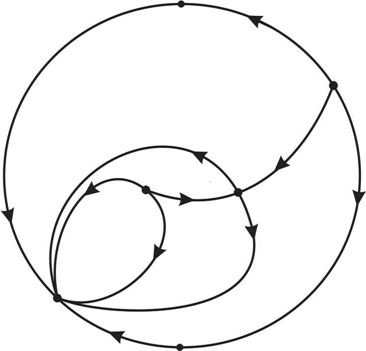
Global phase portrait of system (1.1) on {F3 = 0}.
According to Lemma 2.2 for any trajectory not contained in the invariant surface we have that the ω-limit of any orbit is contained in {F3 = 0} and the α-limit is contained in 𝕊2. The complete phase portrait given in Figure 2 can be obtained with the union of the Figure 6 with the infinity sphere.
Acknowledgements
Partially supported by FCT/Portugal through UID/MAT/04459/2013.
References
Cite this article
TY  - JOUR
AU  - Claudia Valls
PY  - 2019
DA  - 2019/07/09
TI  - On the global dynamics of the Newell–Whitehead system
JO  - Journal of Nonlinear Mathematical Physics
SP  - 569
EP  - 578
VL  - 26
IS  - 4
SN  - 1776-0852
UR  - https://doi.org/10.1080/14029251.2019.1640466
DO  - 10.1080/14029251.2019.1640466
ID  - Valls2019
ER  -