
A simple-looking relative of the Novikov, Hirota-Satsuma and Sawada-Kotera equations
- DOI
- 10.1080/14029251.2019.1640465How to use a DOI?
- Keywords
- Integrable equation; Novikov; Hirota-Satsuma; Sawada-Kotera; Bäcklund transformation
- Abstract
We study the simple-looking scalar integrable equation fxxt − 3(fx ft − 1) = 0, which is related (in different ways) to the Novikov, Hirota-Satsuma and Sawada-Kotera equations. For this equation we present a Lax pair, a Bäcklund transformation, soliton and merging soliton solutions (some exhibiting instabilities), two infinite hierarchies of conservation laws, an infinite hierarchy of continuous symmetries, a Painlevé series, a scaling reduction to a third order ODE and its Painlevé series, and the Hirota form (giving further multisoliton solutions).
- Copyright
- © 2019 The Authors. Published by Atlantis and Taylor & Francis
- Open Access
- This is an open access article distributed under the CC BY-NC 4.0 license (http://creativecommons.org/licenses/by-nc/4.0/).
1. Introduction
Early in the history of integrable systems it was found that there are remarkable transformations connecting different equations [1]. These “hidden connections” abound, and complicate classification attempts, see for example [2]. But, in general, discovery of such a connection is very useful, as typically most of the integrability properties of an equation can be mapped to other related equations. Thus, for example, more research focuses on the KdV equation than on the (defocusing) MKdV equation, and on the NLS equation rather than the many systems related to it by Miura maps (see Figure 1 in [3]). Naturally, the focus tends to fall on the equation in the class which is simplest to write down.
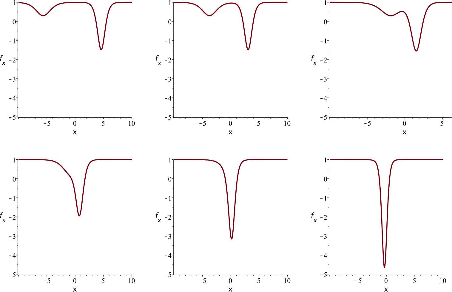
The merging soliton. Parameter values are β = 1 and θ = 1, so λ1, λ2, λ3 ≈ −1.53, −0.35, 1.88. The constants C1, C2, C3 are all taken to be 1. Plots of fx, with f given by (3.1), displayed for times t = −3, −2, −1, −0.5, 0,1.
One of the simple, archetypal equations in integrable systems theory is the Camassa-Holm equation, the first integrable equation to be discovered with peakon solutions [4, 5]. This was followed by the Depasperis-Procesi equation [6,7] and by the Novikov equation [8,9]
In [10] we announced that the Novikov equation is related, by a chain of transformations, to the particularly simple equation
Since the derivation of the various equations in [11] from the Novikov equation is clear, we do not give the full derviation of aN from Novikov here. Proceeding from (1.3), however, make the substitution
Differentiating with respect to x and writing h = rx, so
Modulo rescalings, this is equation (2) in [14], known as the Hirota-Satsuma equation. In [11], Matsuno established the connection between his equation (1.4) and the Hirota-Satsuma equation.
Thus we see that aN is related to the Novikov equation (1.1)–(1.2), the Matsuno equation (1.4) and the Hirota-Satsuma equation (1.6). We note, though, that aN is rather more simple in form than any of these other equations, and thus is surely the natural first object for study. In fact there is a further equation to which aN is related, though this time it is not by a sequence of transformations. We recall that η is an infinitesimal symmetry for (1.3) if, as a consequence of (1.3), f + εη is a solution of (1.3) up to linear order in ε. That is, if
A direct calculation shows that
We have thus seen in this introduction how aN, equation (1.3), is related to numerous equations of interest, but is, at least superficially, the simplest of all. The aim of this paper is to present the basic properties of aN, without reference to any other equation, with the intention that ultimately, aN can be used as a base for study of the other equations. In section 2 we present the Lax pair and Bäcklund transformation (BT) for aN. The Lax pair, which we derived from the Lax pair for the Novikov equation given in [9], is identical to that given for (1.5) in [13]. In section 3 we present the basic soliton solutions of aN, and also solutions describing the “merger” of two solitons, obtained using the BT. However, the BT also gives rise to a solution showing that at least some of the basic soliton solutions are unstable. This limits the possible physical relevance of aN, but on the other hand provides a simple analytic example of the phenomenon of soliton instability, the possibility of which is often overlooked. In section 4 we discuss conservation laws, giving two infinite hierarchies. In section 5 we consider symmetries, but only succeed to give one infinite hierarhcy. We believe a second hierarchy should exist (in parallel to what we have found for conservation laws), but leave this as an open problem. We show the existence of a second infinite hierarchy in the case of the Camassa-Holm equation to demonstrate that this is feasible. In section 6 we show the Painlevé property for aN. In section 7 we discuss a scaling reduction to a third order ODE and give its Painlevé series and the simplest solution. In section 8 we give the Hirota form of aN and a formula for multisoliton solutions. In section 9 we conclude.
Before leaving this introduction, we briefly discuss equation (1.5) that was studied in [13]. As mentioned above, by rescaling t it is possible to replace the constant in (1.3) by any nonzero constant, and thus it is possible to derive properties of the equation (1.5) from those of the equation (1.3) by a limit process. In this way, for example, it is possible to find (several families of) soliton solutions of the (1.5). For a reason that will become clear in the next section, there is a single Lax pair for the equation, irrespective of the value of the constant term. However, in general we are not aware of a process to derive properties of (1.3) from those of (1.5) and we believe the two equations are nonequivalent. Furthermore, it is (1.3) that arises in the context of the Novikov equation. Thus in this paper we study (1.3).
2. Lax Pair and Bäcklund transformation
The Lax pair for aN is
As mentioned above, this Lax pair can be derived, through the necessary transformations, from the Lax pair for the Novikov equation given in [9]. In fact the consistency condition for the Lax pair is not exactly equation (1.3), but rather its x-derivative. This explains why it also provides a Lax pair for the equation (1.5), as studied in [13], and indeed it coincides with the Lax pair given there. The first equation of the Lax pair coincides with the first equation of the Lax pair for SK [17].
The Bäcklund transformation (BT) for aN is
The second equation can be rewritten
The equation (2.4) has appeared before in [18, 19] as part of the BT for SK. The BT (2.4,2.5) is connected to the Lax pair (2.1,2.2) via the substitution
By the relevant transformations, this BT is equivalent to the BT given by Yadong Shang [20] for the Hirota-Satsuma equation.
3. Soliton and merging soliton solutions
Using the standard procedure for finding travelling wave solutions shows that aN has soliton solutions
We call this a soliton solution as the associated profile g = fx of the Matsuno equation (1.4) has a sech2 profile, on the nonzero background β (in fact the profile is −sech2, so it might more correctly be called an antisoliton). Note that here β ≠ 0 and c, the wave speed, are arbitrary, subject to the constraint
So if β is negative, then
Application of the BT (2.3), (2.4), (2.5) to the “trivial” solution
Continuing now to the case that all the three constants C1, C2, C3 are nonzero, if all of them have the same sign then evidently the solution (3.1) will be nonsingular, but if there are differing signs then we expect a singularity. Without loss of generality assume λ1 < λ2 < λ3. Then it can be checked that for θ > 0 the solution with C1, C2, C3 all of the same sign describes solitons of speeds
When C1, C2, C3 have differing signs, various scenarios emerge. Figure 2 shows a case of expulsion of a soliton by a singular soliton. However, the most interesting case is when θ < 0 and the sign of C2 differs from that of C1 and C3. In this case the solution describes the splitting of a left moving soliton into a pair of singular solitons, see Figure 3. For large negative t this solution is a small perturbation of the soliton solution obtained by setting C2 = 0. However, as t increases, the small perturbation grows, ultimately causing a divergence. Thus we deduce that the original soliton solution is unstable. A brief calculation shows this only happens for solitons with
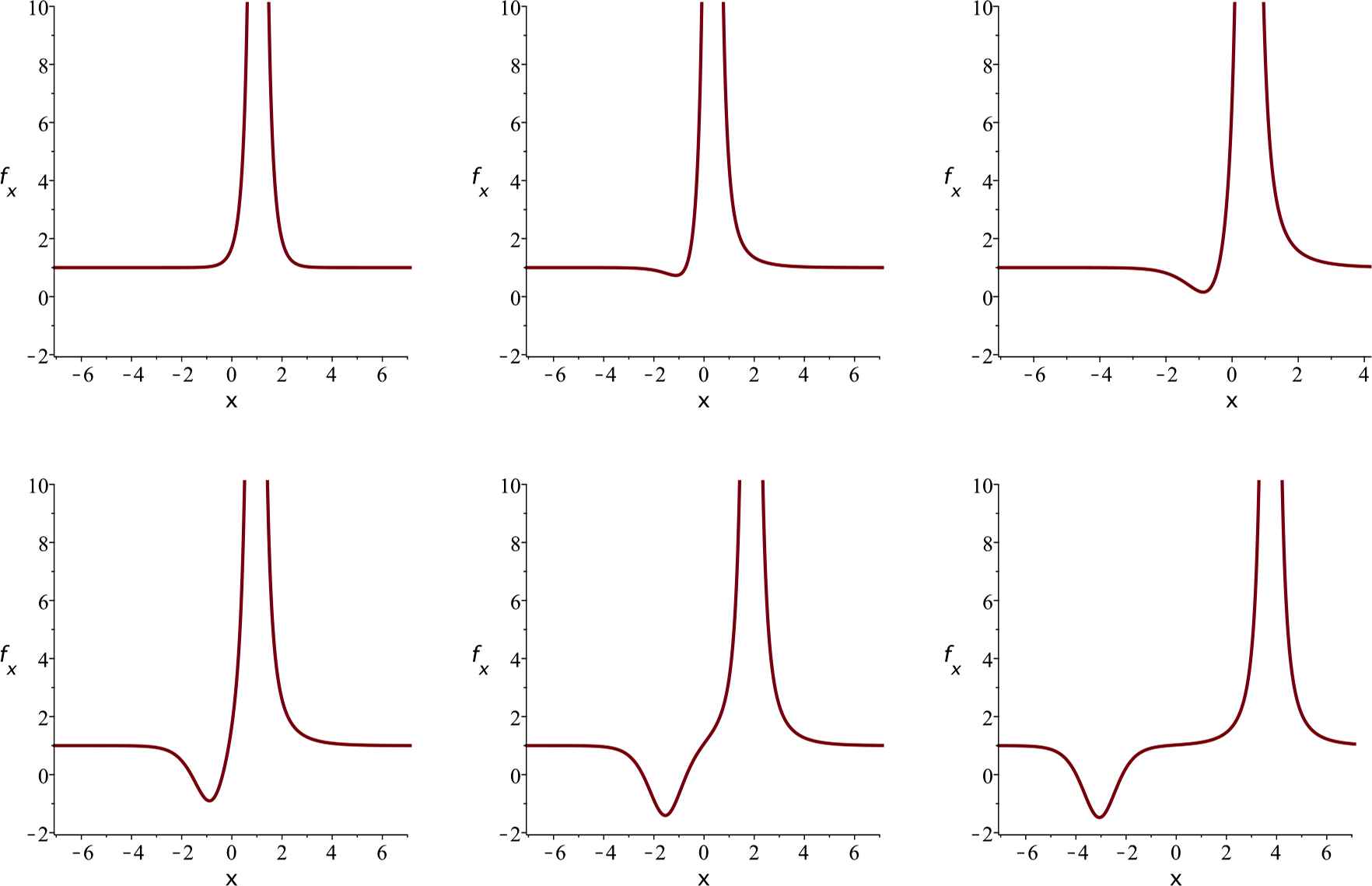
The expulsion of soliton by a singular soliton. Parameter values are β = 1 and θ = −1, so λ1, λ2, λ3 ≈ −1.88, 0.35, 1.53, and C1 = C2 = 1, C3 = −1. Plots of fx, displayed for times t = −3, 0, 0.2, 0.5, 1,2.
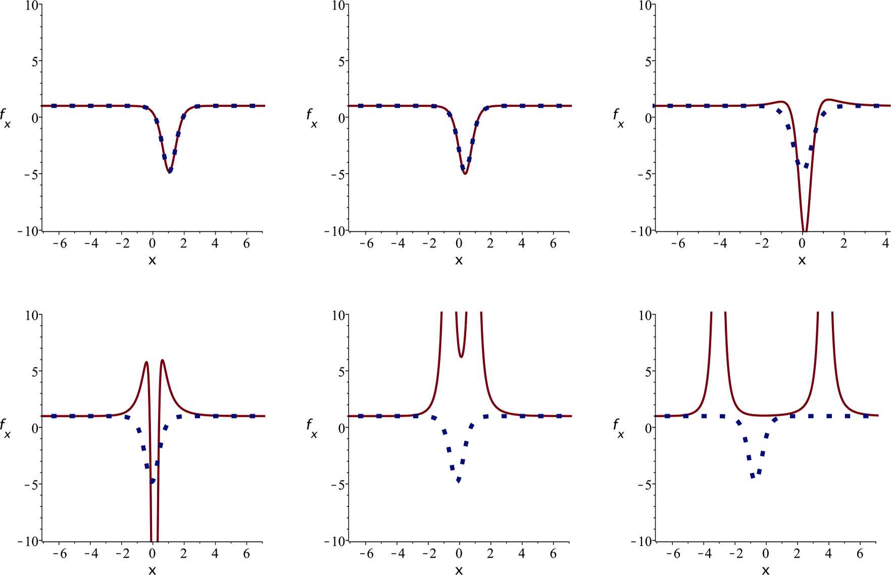
The splitting of a perturbed soliton into two singular solitons. Parameter values β = 1 and θ = −1, so λ1, λ2, λ3 ≈ −1.88, 0.35, 1.53, and C1 = C3 = 1, C2 = −1. Plots of fx, displayed for times t = −3, −1, 0, 0.2, 0.5, 2. The blue, dotted plots show the unperturbed soliton solution, given by the same parameters except C2 = 0.
4. Conservation laws
To find the conservation laws of aN, it is just necessary to observe that (2.6) has the form of a conservation law. Thus v, which is the solution of (2.4)–(2.5) and depends on θ, provides a generating function for (densities of) conservation laws. Similar to what was observed for the Camassa-Holm equation in [22], this can be expanded in various different ways to obtain series of conservation laws.
For large |θ|, the solution v to (2.4) can be expanded in an asymptotic series of the form
Each of the coefficients vi is the density for a conservation law. The first few coefficients are given as follows:
Further terms can be computed using the recurrence relation
So, for example
Here f5x, f6x,... denote 5th, 6th etc. derivatives of f with respect to x. For each i = 1,2,... vi, is the density F of a conservation law Ft + Gx = 0. For i = 1,2,3,4,6 the conservation laws are evidently trivial (F = Hx, G = −Ht for some H). For i = 5,7 we obtain the following conservation laws (after eliminating trivial parts):
Note that there are 3 possible series for v, corresponding to the 3 possible choices of v−1. The dependence of v1, v2,... on the choice of v−1 is clear, and can be verified to be consistent with the recursion relation. We denote the three associated asymptotic series by v(1), v(2), v(3). If we define σ = v(1) + v(2) + v(3), then σ has asymptotic series
It follows that v3i is a total x derivative for all i, and the associated conservation laws are trivial. We also conjecture that v2i is a total x derivative for all i, though do not yet have a direct proof of this.
Another possible expansion of v, this time for small |θ|, is
The coefficients of this series are obtained by plugging (4.4) into (2.5), and involve derivatives with the respect to t, which can not be eliminated. We call it the “expansion in the t direction”, as opposed to the (4.1) which is the “expansion in the x direction”. The first few coefficients of (4.4) are
For each i = 1, 2,..., wi is the density of a conservation law. The conservation law arising from w2 is trivial, but from w1, w3, after elimination of some trivial parts, we obtain the following conservation laws:
5. Symmetries
By the direct computation of the first order generalized symmetries [23] of aN we obtain
Following the ideas of [24], and with some inspiration from formulas that appeared in [10, 21], it is possible to find a generating function for symmetries of aN in terms of mulitple solutions of the BT (2.4)–(2.5):
Here A is defined by (4.2). It is straightforward to check directly that η = Q satisfies the linearized aN equation
To generate local symmetries for aN from (5.1) we take v(1), v(2), v(3) to be given by the 3 possible asymptotic expansions of v of form (4.1), as given in the previous section. Substitution of these asymptotic expansions into Q and expansion in inverse powers of θ1/3 gives an infinite hierarchy of symmetries. The first two symmetries in this hierarchy are η(f), η(x). From the higher order terms we obtain
Observe that η(5) defines the potential Sawada-Kotera flow (1.7).
We have not succeeded in using the second expansion (4.4) of v in (5.1) to generate a second hierarchy of symmetries, as the coefficients in this expansion are unique. However, we note that there are other equations for which such an approach is possible. Specifically, for the Camassa-Holm equation
One possible expansion of s, the “expansion in the x direction”, is in the form
There are two versions of this expansion (related by replacing α1/2 by −α1/2), and these were used in [25] to construct a hierarchy of symmetries. However there is also an “expansion in the t direction”:
The first few coefficients are
Once again, there are two versions of this expansion, corresponding to the choices s0 = ±1. A generating symmetry for the Camassa-Holm equation was found in [25] and its form is
In [25] the two expansions of s of form (5.6) were used in this formula to produce a hierarchy of symmetries. A second hierarchy is found by using the two expansions of form (5.7). The first few symmetries we get are
This hierarchy of symmetries is different from the one found in [25]. We note that this is a hierarchy of hyperbolic, not evolutionary, symmetries. These symmetries have already been found, for example, in [26]. The existence of hierarchies of such symmetries has been also discussed in [27]. In parallel to the fact that we have been able to find two hierarchies of conservation laws for aN, we expect there to be two hierarchies of symmetries. But finding the second hierarchy remains an open problem.
6. Painlevé Property
It is lengthy, but straightforward, to verify that aN has the WTC Painlevé property [28]. There are formal series solutions about the singularity manifold ϕ (x,t) = 0 of the form
7. Scaling Reduction
aN has the obvious scaling invariance f → λ f, ∂x → λ∂x, ∂t → λ−3∂t. Thus we look for a reduction to an ordinary differential equation by taking
This gives the third order equation
This equation has the Painlevé property, with a pole series
Note that if F satisfies the third order equation (7.1) then E is constant. But in the other direction, E being constant implies that either F satisfies the third order equation (7.1) or F = C1 +C2z3/2 where C1, C2 are constants. Remarkably, the functions
By the substitution
This is a special case of equation SD-I.b, equation (5.5) in [30], which can be solved, as explained in [30], in terms of either Painlevé III or Painlevé V transcendents.
8. Hirota form
Substituting
See, for example, [31] for notation. This has an unusual form, in that as far as we are aware, most studies of equations in Hirota form assume the form P(Dx, Dt,...)ϕ · ϕ = 0 with P(0, 0,...) = 0 (see, for example, [31], equation (17)). However, by substituting
Modulo rescalings, this is the Hirota form of the Hirota-Satsuma equation [31–33]. The basic soliton solution is
As observed in our previous discussion of soliton solutions, the speed c is restricted by the requirement
Here we have written the phase shift factor A in a form in which it is clear that at least in the case that both c1 and c2 are positive, A is positive, thus guaranteeing a non-singular two soliton solution of aN. Note that for certain values of the parameters A can either vanish, or be ill-defined, as the denominator vanishes. It can be checked that this happens if and only if
In this case the two soliton solution reduces to the “merging soliton” solutions described in section 3. The two soliton solution extends to multisoliton solutions in the usual way for integrable equations of KdV type [31,32]. So, for example, the three soliton solution is, in the obvious notation,
We have not yet succeeded in determining whether there exist nonsingular superpositions of merging solitons and regular solitons.
9. Conclusion
In this paper we have researched the aN equation, an integrable nonlinear equation, which is notable for taking a particularly simple form, with just a single, quadratic nonlinear term, and for having relationships with various other significant integrable equations. Among the interesting properties of this equation we would mention the existence of merging solitons, the fact that some of the soliton solutions are unstable, which can be demonstrated very effectively, and the existence of two infinite hierarchies of conserved quantities. Among the matters that we have not been able to resolve fully and which merit further research, we would mention the lack of a superposition principle for the Bäcklund transformation, the need to establish the stability of other solutions, and the need for a fuller exploration of the space of solutions, particularly to determine if there are nonsingular ways to superpose merging solitons. Also, we have only been able to give a single hierarchy of local symmetries so far. We note that the aN equation is not in evolutionary form, which limits its potential application; but its superficial simplicity and rich properties make it notable, nonetheless.
References
Cite this article
TY  - JOUR
AU  - Alexander G. Rasin
AU  - Jeremy Schiff
PY  - 2019
DA  - 2019/07/09
TI  - A simple-looking relative of the Novikov, Hirota-Satsuma and Sawada-Kotera equations
JO  - Journal of Nonlinear Mathematical Physics
SP  - 555
EP  - 568
VL  - 26
IS  - 4
SN  - 1776-0852
UR  - https://doi.org/10.1080/14029251.2019.1640465
DO  - 10.1080/14029251.2019.1640465
ID  - Rasin2019
ER  -