
An exact solution for geophysical internal waves with underlying current in modified equatorial β-plane approximation*
- DOI
- 10.1080/14029251.2019.1640468How to use a DOI?
- Keywords
- Geophysical internal waves; modified β-plane; exact solution; mean velocity; mass flow; Lagrangian variables
- Abstract
In this paper, a modification of the standard geophysical equatorial β-plane model equations, incorporating a gravitational-correction term in the tangent plane approximation, is derived. We present an exact solution to meet the modified governing equations, whose form is explicit in the Lagrangian framework and which represents internal oceanic waves in the presence of a constant underlying current. It is rigorously established, that the solution is dynamically possible, by way of analytical and degree-theoretical considerations. In the sense that the mapping it prescribes from Lagrangian to Eulerian coordinates is a global diffeomorphism. In addition, the paper an analysis of the mean flow velocities and related mass transport are presented in this paper, they are induced by certain geophysical internal waves. In particular, we examine an exact solution to the geophysical governing equations in the modified β-plane approximation at the equator which incorporates a constant underlying current.
- Copyright
- © 2019 The Authors. Published by Atlantis and Taylor & Francis
- Open Access
- This is an open access article distributed under the CC BY-NC 4.0 license (http://creativecommons.org/licenses/by-nc/4.0/).
1. Introduction
In the paper, we aim at discovering an exact solution for internal geophysical waves with an underlying current in modified β-plane approximation. The equatorial region is characterised by a thin, permanent, shallow layer of warm and less dense water overlying a deeper layer of cold water, both of constant densities. The two layers separated by an interface called the thermocline [2]. Our aim is to investigate the flow induced by the motion of the thermocline by presenting an exact solution which models internal geophysical waves propagating in the presence of an underlying current.
Although immense topographical and climatological differences, the Atlantic Pacific and Indian Equatorial Oceans present a peculiar dynamics compared to off-equatorial regions. Concerning their mean flow, internal geophysical waves field is considered to be anomalous, despite high levels of internal wave energy and shear, mixing appears to be weaker than at the middle latitude [17, 20]. On the other hand, strong, zonal, basin-scale currents is the Equator’s characteristic, known as the Equatorial Deep Jets, presenting a very complex temporal, meridional and vertical structure.
In this study observations collected in the deep Equatorial West Atlantic Ocean (Fig.1) are used to characterize and understand the peculiarities of the equatorial belt over the whole frequency spectrum. The dataset consists of approximately 1.5 year long time series of current velocities, measured acoustically and with current meters, moored between 0° and 2.5°N, at 38°W, off the Brazilian coast. The time series cover the whole water column, even if not continually. The complete depth range is captured by means of a quasi synoptic CTD/LADCP meridional transect, where the anisotropy of the equatorial mean flow field is evident.
In particular, we want to investigate the possible presence and role of internal wave trapping and focusing in determining the equatorial ocean dynamics that may drive zonal mean flows due to mixing of angular momentum, as suggested in [37]. We can observe the strong and highly coherent zonal mean flows not only in the oceans but also in the equatorial regions of fluid planets, it suggests that their existence could be more likely related to general properties of these systems such as shape, stratification and rotation, rather than to local weather systems.
Internal geophysical waves that travel within the interior of a fluid, the wave propagate at the interface or boundary between two layers with sharp density differences. Internal waves are in fact present in all kinds of stratified and rotating fluids, and are thought to play a key role in diapycnal mixing, because of their oblique propagation, geometric focusing and angular momentum mixing, with consequent triggering of significant zonal flow. Moreover, recent ray tracing studies [37, 40] have shown that the equatorial regions of stratified and rotating spherical shells (such as our ocean) are possibly affected by instabilities due to internal geophysical waves location, at places where the simplest shaped and most energetic internal geophysical waves attractors occur.
Many literatures research the exact, nonlinear solution for equatorial ocean waves propagating eastward, in the layer above the thermocline and beneath the near-surface layer in which wind effects are noticeable, in Constantin (2013) described recently it. The solution was obtained in Lagrangian coordinates by adapting to the setting of equatorial geophysical waves in the β-plane regime the celebrated deep-water gravity wave obtained by Gerstner (1809) and Constantin (2011) for a modern exposition of the flow induced by Gerstner’s wave; Pollard (1970) for a modification describing deep-water waves in a rotating fluid, and Constantin (2012) and Henry (2013) for equatorially trapped surfaced water waves, the main features of the flow described in Constantin (2013) are that each particle remains at the same latitude, describing a circular motion so that overall the equatorially trapped wave motion is symmetric about the equator, it represents at each fixed latitude an eastward-traveling wave whose amplitude decays with the meridional distance from the equator. An explicit solution was discovered in Lagrangian variable for the full water wave equation in 1809 Gerstner [18]. This is one of only a handful of explicit solutions to the governing equations which have been constructed Gerstner’s wave is a two dimensional gravity wave where Coriolis effect are neglected and where the motion is identical in all planes parallel to the fixed vertical plane, [3,4,21] analyse this exact solution and [5,42] extend to describe three dimensional edge-waves propogating over a sloping bed recently, we can obtain some exact solution describing nonlinear equatorial flow in the Lagragian framework, Gerstner [18] found the solution in Lagrangian coordinates for periodic in a homogenous fluid, and the solution was rediscoveryed by Rankine [39], Constantin [3,4], Henry [21] offer a modern treatment of Gerstners wave. This flow has been used to describe a number of interesting studies within the class of gravity edge wave (cf Ehrnstorm.et.al [14], Henry and Mustafa [30], Johson [33], Constantin [5], Stuhlmeier [42], Matioc [36], Hsu [27]). In Constantin [6] equatorially trapped wind waves were presented, see also Constantin and Germain [10], and Hsu [27]. In Constantin [7] internal waves describing the oscilation of the thermocline as a density interface separating two layer of constant density; with the lower layer motionless, were presented in the β-plane approximation. In Constantin [8] demonstrated that the f-plane approximation is physically realistic for contain equatorial flow. In [6] achieved successfully an exact solution for geophysical water waves incorporating Coriolis effects. This solution is Gerstner-like in the sense that setting Coriolis terms to zero recovers the Gerstner wave solution. However, the wave solution derived in [6] is a significant extension of Gerstener’s wave for a number of reasons. For example, it is three-dimension and equatorially trapped, where by Coriolis terms play a vital role in the decay of wave oscillations aways from the equator subsequently a variety of exact and explicit solution were deduced and illustrated in various papers, including solution with underlying background currents [15, 19, 22, 28].
This paper is motivated by the article [11–13]. When Constantin presented explicit nonlinear solution for geophysical internal waves propagating eastward in the layer above the thermocline and beneath the near-surface layer in which wind effects are predominant. What’s more, we remark that while β-plane approximation is regarded as reasonable for large-scale ocean graphical considerations, nevertheless from a mathematical modeling perspective it is lamentable that an appreciable level of mathematical detail and structure is lost from the model equations as a result of the flattening out of the earth’s surface. Within the vast literature investigated a lot of interesting mathematical approaches which aim to retain some of this structure in modelling equatorial waves (cf. [11–13, 23]). The primary purpose of this paper is to preserve the geometric artifacts of the earth’s curvature by introducing a gravity correction term into the standard β-tangent plane model, it can result in the modified governing equations (3.3).
The paper is organized as follows: Section 2 presents the general governing equation in β-plane approximation. Section 3 introduces the governing equation in modified β-plane approximation. Section 4 analyses the model of this paper in different layers and recommends the governing equations in modified β-plane approximation for each layer. Section 5 provides an exact nonlinear solution for internal geophysical waves. The solution is showed in Lagrangian coordinates by describing the circular path of each particle.
2. Preliminaries
We researched the flow model is symmetric about the equator, being confined to a region of overall width of about 200 km. We now present the governing equation for geophysical water waves in equatorial regions. We consider geophysical water waves propagating in the Equatorial region on an incompressible, inviscid fluid. Assuming that the earth is a perfect sphere of radius R = 6378km. This sphere rotates around the axis through the north and south poles with a constant rotational speed ω = 73 × 10−6rad/s. We think about surface water waves propagating zonally in a relatively narrow ocean strip less than a few degree of latitude wide, the coriolis parameters were took:
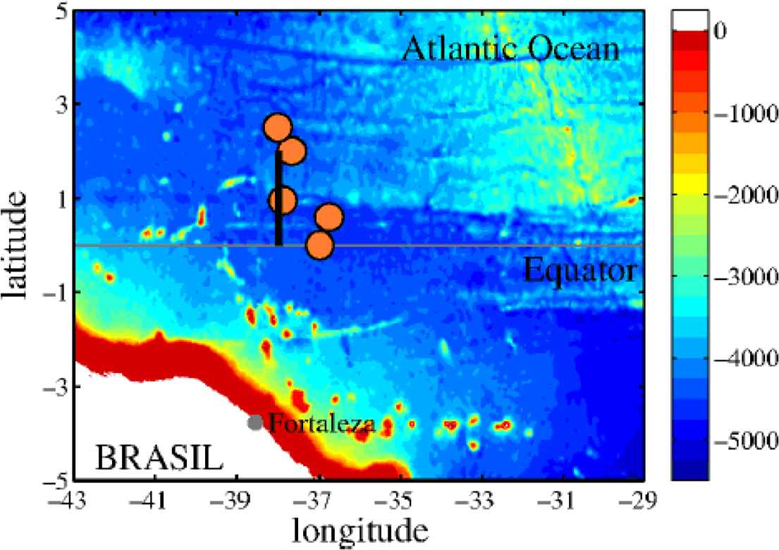
Study area. Circles: approximately 1.5 year long moorings, thick line:CTD/LADCP transect.
The β-plane effect is merely the result of linearizing the Coriolis force in the tangent plane approximation: under the assumption that equatorial meridian has moderate distance, we may use the meridional distance define y, the approximations sinϕ ≈ ϕ and cosϕ ≈ 1 could be used giving what is called the equatorial β-plane approximation in which the Coriolis force:
It is permissible that a Taylor expansion approximation of the Coriolis force near the equator. Although the Earth was assumed to be a flat sphere, if the spatial scale of motion is adequate, then the region occupied by the fluid can be approximated by a tangent plane. The linear term of the Taylor expansion yields the β-plane effect βy noticeable in equation (2.5).
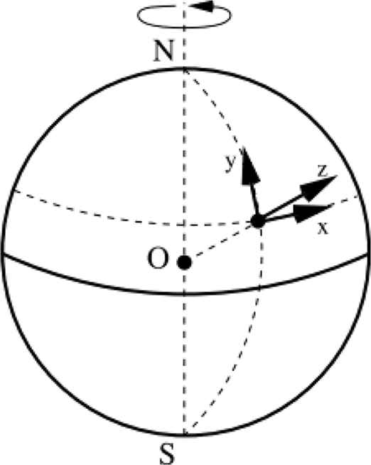
The rotating frame of reference: the x-axis is chosen horizontally due east, the y-axis is chosen horizontally due north and the z-axis upward.
3. Modified equatorial β-plane equation
The full governing equation (2.1) is changed into the vector formal:
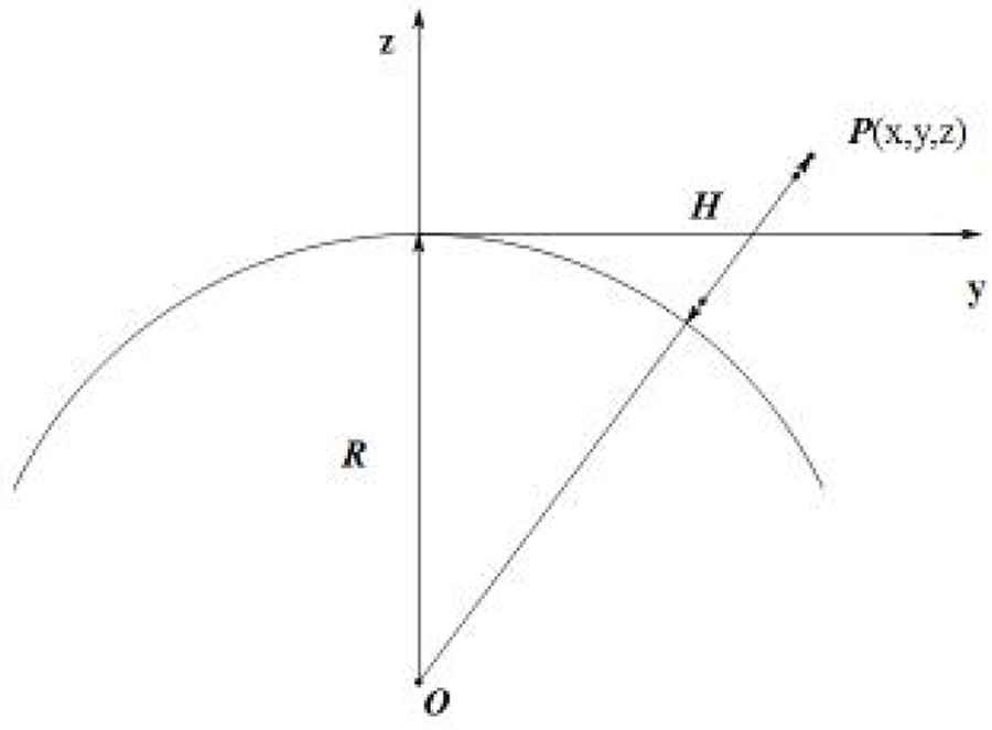
We take into account F of the equation (2.1), in thinking the form that the gravitation body force F gets in our approximation. We accommodate a correction term that includes the deviation of the tangent plane from the earth’s curved surface as follows. We think about the point P in Fig.3 and its distance from the earth’s center o is
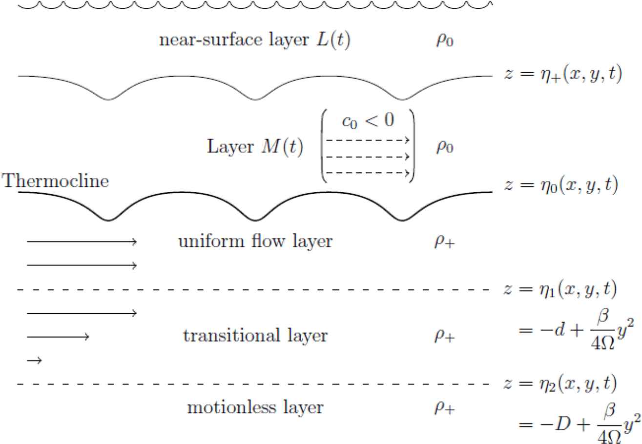
Depiction of the main flow region at fixed latitude y. The thermocline is describes by a trochiod propagating eastward at constant speed. The thermocline separates two layer of different densities ρ0 < ρ+ in stable stratification and c0 represents the constant underlying current term in M(t). Typical equatorial depth values are d = 160 m and D = 200 m, with a near-surface layer L(t) of average depth 60 m and with a mean depth level of about 120 m for the oscillations of the thermocline.
Therefore we can simplify the full governing equation (3.1) into
4. Analysis of the Model
The principle objective of this paper is to present an exact solution to (3.3) which describes eastward propagating equatorially trapped waves (with constant wavespeed c > 0) in the presence of a constant underlying current c0, which for the present time may be either positive or negative. The initial model is investigated a Gerstner-like internal waves as part of two layer hydrostatic model in [7], a physical complex multilayered, non-hydrostatic model was successfully derived for internal waves in Constantin [9], A diagrammatic sketch for the model is given in Fig. 3, and it may be described as follows.
Schematic of tangent plane approximation
L(t) denotes the upper near-surface region of the ocean where wind effects are important, and we assume that the wave motion there is a small disturbance in oceanic dynamics, which is mainly controlled by wind and waves. Thus we consider that the motion of internal geophysical waves does not play a major role in the flow characteristics of fluids in L(t), and so for the purpose of this model we will not discuss the interaction between geophysical waves and wind waves in this L(t) region. Beneath L(t), whose lower-boundary the propagation, we can label z = η+(x, y, t), We assume that fluid motion is mainly caused by fluctuations caused by thermocline propagation, which we denote z = η0(x, y, t), interacting with a uniform underlying current c0, M(t) label this region between the interfaces η+ and η0. The appearance of the constant current in our model takes an apparently simple form in the Lagrangian setting, but both mathematically and physically it leads to highly complex modifications in the underlying flow.
Next we suppose that the fluid has a constant density ρ0 in the region above the thermocline η0, where the fluid has constant density ρ+ > ρ0 beneath the thermocline—indicative values for the density difference are given by
We divide the high density fluid field below the thermocline into three separate regions, which transform the fluid motion induced by the propagation of the thermocline to a static deep–water region. In the region bounded above by the thermocline and below by the interface z = η1(x, y, t) the flow is uniform with velocity (c − c0, 0, 0), where c > 0 is the propagation velocity of thermocline oscillation. The region between z = η1(x, y, t) and z = η2(x, y, t) is a transition layer where the fluid motion decreases until we reach the deep-water layer beneath the interface z = η2(x, y, t) where it is completely still. We show the form of the governing equation (3.3), which are related to each layer, and then we derive exact solution to these equations.
- 1.
The layer M(t)
In the area η0(x, y, t) < z < η+(x, y, t) we seek a solution of the governing equation (3.3) which take the form
equip with the incompressible conditionand the kinematic boundary conditionon - 2.
The layer of uniform flow
Between the boundary η1(x, y, t) < z < η0(x, y, t) we look for a solution of
together with the incompressible conditionand the kinematic boundary conditionon - 3.
The transitional layer
In the region η2(x, y, t) < z < η1(x, y, t) the form of the governing equation is the same as above:
equip with the incompressible conditionand the kinematic boundary conditionon - 4.
The motionless deep-water layer
In the district z < η2(x, y, t) the form of the governing equation as follow :
and we have always assumed that water is static, thus
We want to successfully implement the multi-layered model described above, each equation must be coupled with the continuity of pressure at each interface. We also note the boundary conditions of motion
5. Exact solution
In this section, we defined an exact solution of the governing equation (3.3). The exact solutions satisfying the above multi-layered model are given. Because the flow characteristics of various solutions vary greatly. To facilitate demonstration, we describe the solution layer by layer, working from the bottom upwards.
- 1.
The motionless deep-water layer
For certain fixed equatorial depths D > 0, we set
for - 2.
The transition layer
For some fixed equatorial depth d < D, we set
Then the equations (4.6) are simplified to
which yieldsNote that the pressure P and the velocity u are continuous across the interface z = η2(x, y, t).
- 3.
The layer beneath the thermocline
The interface z = η0(x, y, t) represents the oscillating thermocline, and for every latitude y it is an eastward-propagating travelling wave form. In the area η1(x, y, t) < z < η0(x, y, t), we set the flow to be uniform with u = c − c0 and v = w = 0. The reduced vertical momentum equation writes
and the y-momentum equation can writeso we haveThe continuity of pressure across the interface z = η1(x, y, t) be required in the region. Evaluating the pressure (5.2) and (5.3) on
- 4.
The layer M(t) above the thermocline
In the section, We show the exact solution in the M(t) layer, which represents the wave propagating along the longitudinal direction at a constant propagation speed c > 0, in the presence of a constant underlying current of strength c0. A clear description of the process facilitates the use of the Lagrange framework [1]. Let us rewrite the governing equation (3.3) in the following form
The Lagrangian position (x, y, z) of fluid particle are given as functions of the labelling variables (q, r, s) and time t by
For simplicity, let us choose
We also require
From a direct differentiation of the system of coordinates in (5.6) the velocity of each fluid particle may be expressed as
Accordingly to above statements (5.5) can be converted into
The change of variables
Now a suitable pressure function be prescribed such that (5.12) holds. We can eliminate terms containing θ in (5.12) and we can suppose
Note that we make a natural assumption that the pressure in M(t) has continuous second partial derivatives, and thus Psr = Prs implies that
Which leads to the expression for
Now the gradient of the expression
With (5.14) and f(s) we get
Comparing the respective pressures at the thermocline (5.16) and (5.18) and examining the time dependent θ terms. It follows that the continuity of the pressure across the thermocline requires
Following (5.19), a comparison of (5.16) and (5.18) with regard to the continuity of pressure across the thermocline brings about the expression
5.1. Admissible value of the underlying current c0
In order to complete our presentation, we must consider the values of the current c0 the flow is possible for hydrodynamics, we can find a unique r0(s) such that (5.20) holds. For each fixed s ∈ [−s0, s0] the mapping
Then r0(s) determines the thermocline. The constant
We make enforce the restriction that the function r0(s) is strictly decreasing with s, which corresponds to the scenario present in [9] for the setting c0 = 0. Thus we get
The relation (5.24) holds for all values c0 ≤ 0. Specific to our setting, equation (5.24) provides a bounded for positive values of the constant underlying current c0. By the implicit function theorem, r0(s) is even and smooth function. so we can say that the function s → r(s) decrease as s increase. We note that (5.24) indicates that the average depth of the thermocline [d0 − r0(s)] increase slightly with the distance from the equator at every latitude s, while the boundary rise of transitional layer. This means at some latitude the two regions will intersect, resulting in a more complex flow.
In order to complete the solution, it is still necessary to specify boundaries that define the two layers M(t) and L(t). This can be obtained by choosing some fixed constant
The previous consideration indicate that β0 determines a unique r+(s) > r0(s). The function s ↦ r+(s) has the same features as the function s ↦ r0(s). It is even, smooth and strictly decreasing for |s| > 0. Setting r* = r0(s), we ensure condition (5.7). This completes the proof that (5.6) is the exact solution of the governing equation (4.1)–(4.3) of internal water waves propagating in presence of constant underlying current.
Remark 5.1.
It has recently rigorously shown in [43] that the internal wave solution considered in [9] is dynamically possible. These considerations are also applicable to models containing the constant underlying current shown in this paper.
Remark 5.2.
In this paper, it is assumed that the model describes the fluid with a static deep water fluid layer.
5.2. The vorticity
We can compute the inverse of the Jacobian matrix (5.8) as
5.3. The dispersion relations
The relation (5.19) determines the dispersion relationship of flow by regarding (5.19) as a quadratic c. To solve it, we obtain that
- 1.
If c0 > 0, the velocity c can take positive and negative values, unlike the case of the f-plane approximation. If c is take positive, the uniform current c − c0 will flow eastward when c0 is small than
- 2.
If c0 < 0, the existence of a real velocity c requires
- 3.
If c0 = 0, the oscillations of the thermocline described propagate eastwards in the shape of trochoid, and each particle in the layer M(t) describes a counting clockwise circular vertical closed path with reduced diameter as we rise above the thermocline. The wave motion in M(t) induced by the propagation of the thermocline, as described by the solution (5.6), is equatorially -trapped and (5.15) is a suitable choice for the function f(s).
5.4. Global validity of (5.6)
We can have far proven that the mapping from Lagrangian coordinates to Eulerian coordinates (5.6) is compatible with the governing equation in the modified β-plane. We provide rigorous mathematical proof that it is dynamically possible to prescribe the flow. If we can show that the mapping (5.6) is a global diffeomorphism between D to the fluid domain. This ensure (5.6) describe a three-dimensional, nonlinear motion of the entire fluid body is possible, so that fluid particles will not collide in the M(t) layers.
We want to prove that the mapping (5.6) is a global isomorphism. We can simplify matters by setting of t = 0, generally, we can recover by changing variables (q, s, r) ↦ (q + ct, s, r) coupled with translating the x-variable by (c0 + c)t. we define the operator
Lemma 5.1.
The map
Proof.
The inequality r > 0 ensure that the Jacobian matrix (5.8) has a non-zero determinant throughout
5.5. Mean Velocities and Stokes Drift
In this section, the effects of constant undercurrent on both the average Lagrangian and Eulerian velocities caused by the exact solution (5.6) are analyzed. In [10] shown that in the absence of a current, that is to say c0 = 0, the mean Lagrangian velocity is zero and the mean Eulerian velocity flows westwards. However, in the absence of the current, the Stoke Drift is the difference between the mean Lagrangian and Eulerian velocities [34, 35], is eastwards, we find that the situation is much more complicated in the presence of undercurrent, especially in determining the average Euler velocity.
5.5.1. Mean Lagrangian Flow velocity
The mean Lagrangian flow velocity at a point in the fluid domain is the mean velocity over a wave period of a marked fluid particle which originates at that point. Thank to the Lagrangian description of an exact solution (5.6). In the region M(t), it is easy to obtain the horizonal mean Lagrangian velocity over a wave period
5.5.2. Mean Eulerian Flow Velocity
When working in the Eulerian setting, matters are greatly complicated due to the existence of underlying current, the mean Eulerian flow velocity at a fixed point in the fluid domain is the Eulerian fluid velocity at that fixed point averaged over a wave period. In the case of the velocity field (5.9), we can take the mean over a wave period of the horizontal velocity (the first equation of (5.9)) to compute the mean Eulerian flow velocity at any fixed depth beneath the wave. An explicit solution can be obtained for the equation describing ocean waves is an extraordinary achievement. In our case, it is possible to use Lagrangian formulation, however, compared with the more extended analysis in fluid dynamics, the study of these kind of flows follows from an Eulerian approach, and in order to find the Stokes drift, we determine the mean Euleian velocity. In this framework, the observer focus on the fluid motion, for a fixed location (x, y, z) as the time passes, we can discover the horizonal mean Eulerian velocity over a wave period T, it is given by
We note from (5.40) that whenever sinθ = 0, α is maximised or minimised with respect to q, for a fixed depth z0. The maximal and minimal values achieved by α are given implicitly by the relationes
By differentiating x in (the first equation of (5.6)) with respect to q, using (the first equation of (5.9)) and taking into account (5.40). We obtain
Therefore, we can give the mean Eulerian velocity relation as follows
The existence of a non-zero undercurrent of c0 adds an important complication to the expression (5.45), especially that the symbols of the average Euler velocity are usually difficult to distinguish from the above expression. However, depending on the size and direction of current c0, we may obtain estimates for determining the direction of the mean Eulerian velocity following from the inequalities
5.5.3. Mean Eulerian Flow Velocity
First, we study the case that represents an underlying adverse current in the Lagrangian variables, when c0 is positive, the second integral term on the right-hand side of inequality (5.45) satisfies
From (5.24) can get 0 < c0 < c, equation (5.47) yields
Accordingly, the mean Eulerian flow velocity is westwards for all admissible values of c0. In order to obtain the range of the mean Eulerian flow, we note that
Since ξ ≥ kr* > 0 then −ξ ≤ −kr* < 0, we see that the mean Eulerian flow velocity is in some range for all latitude s and depth z0, the range as follows
It is not surprising that the mean Eulerian flow is westward for an adverse current. In the absence of the current, the mean Eulerian flow is westward [10] and the existence of the adverse current term in (5.45) only exacerbates this effect.
5.5.4. The case c0 ≤ 0
The case deputies an underlying following current when c0 is non-positive (c0 ≤ 0). In this case, the effect of current on the average Euler current in (5.45) is complex and difficult to distinguish. Generally, the influence can not be determined directly from the expression (5.45). However, some broad characteristics of the flow can be deduced by working as follows. The mean Eulerian velocity (5.45) is westwards (〈u〉E < 0), if
This series of inequalities holds and accordingly 〈u〉E < 0, if
We note that in the absence of an underlying current(c0 = 0), so the average Eulerian velocity in the westerly direction is obtained, it is consistent with observation of [18]. The Eulerian flow (5.45) is eastwards, that is 〈u〉E > 0 if
This series of inequalities holds, and accordingly 〈u〉E > 0 if
5.6. Stokes Drift
The Stokes Drift (or mean stokes) velocity us(z0) is define [27] by the relation
For an adverse current c0 ≥ 0. From (5.24) that, we have
Therefore, the stokes drift is eastwards throughout the domain for c0 ≥ 0. The Stoke drift expression is more complex and difficult when the current is c0 < 0. However, we remark that for c0 < 0, if the current has the magnitude of (5.53). So the stokes drift must be westwards.
5.7. Mass flux
Finally, we briefly discuss the mass transport properties of fluid (5.9), in which we recall that 〈u〉L, as the average velocity of the labeled particle, is sometimes called mass transport velocity. For a nonzero underlying current (c0 ≠ 0), we intuitively antipate the mass flux between two given latitudes y1 and y2 through a fixed plane x = x0 in the layer of application of the modified β-plane approximation. The relative mass flux between those fixed latitudes in the region of M(t) defined by the thermocline z = η0(x, y, t) and interface z+ = η+(x, y, t) is x = x0, we can give as follows
We can use the lagrangian labelling variables to transform this expression (5.55), The implicit function theorem ensures that x = x0 is fixed in the expression.
Then, we can find s1 and s2 satisfies α2(s1) = β2(s1) = y1 and α2(s2) = β2(s2) = y2 by (5.57) for every latitude y, and Fubini’s Theorem can be used in the domain of integration, the mass flux becomes
For the plane x = x0, the meridional mass flux is cancelled out, resulting in a mass flux that depends on the latitude amplitude from y1 to y2.
6. Discussion and Outlook
In this paper, we have investigated the exact solution for geophysical internal waves in different layers. The geophysical internal waves should satisfy density stable fraction and have disturbed energy sources. Further more, we have given the expression of the exact solution in different layers, and we want to find the effect of correction term on solution. First, we discusses the effect in the motionless deep-water layer.
In Fig. 5, y′ and z′ parallel to the rotating coordinate frame y-axis and z-axis, respectively. θ represents the angle with z′ at different times. After simple mathematical calculation. We know that there is always a
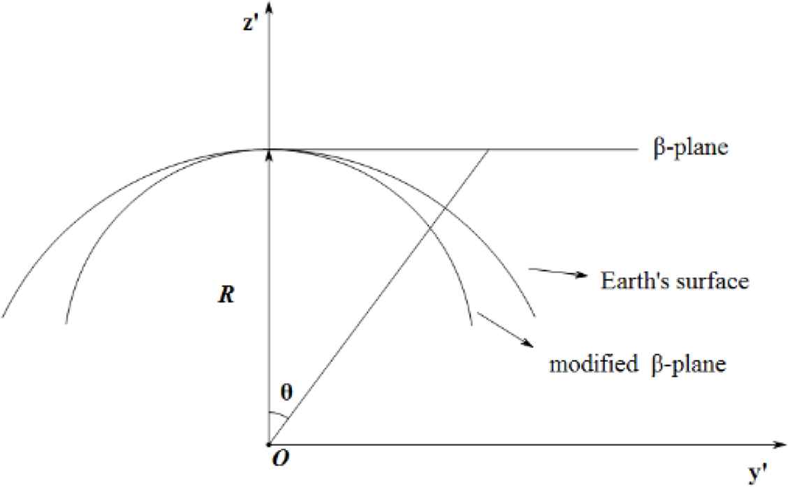
Analysis of plane approximation.
In the future, we will investigate stability of the exact solution in modified β-plane.
Footnotes
The work is supported in part by a NSFC Grant No. 11531006, PAPD of Jiangsu Higher Education Institutions, and the Jiangsu Center for Collaborative Innovation in Geographical Information Resource Development and Applications.
References
Cite this article
TY  - JOUR
AU  - Dong Su
AU  - Hongjun Gao
PY  - 2019
DA  - 2019/07/09
TI  - An exact solution for geophysical internal waves with underlying current in modified equatorial β-plane approximation*
JO  - Journal of Nonlinear Mathematical Physics
SP  - 579
EP  - 603
VL  - 26
IS  - 4
SN  - 1776-0852
UR  - https://doi.org/10.1080/14029251.2019.1640468
DO  - 10.1080/14029251.2019.1640468
ID  - Su2019
ER  -