
Final evolutions of a class of May-Leonard Lotka-Volterra systems
- DOI
- 10.1080/14029251.2020.1700635How to use a DOI?
- Keywords
- May-Leonard system; Lotka-Volterra system; invariant, global dynamics
- Abstract
We study a particular class of Lotka-Volterra 3-dimensional systems called May-Leonard systems, which depend on two real parameters a and b, when a + b = −1. For these values of the parameters we shall describe its global dynamics in the compactification of the non-negative octant of ℝ3 including its infinity. This can be done because this differential system possesses a Darboux invariant.
- Copyright
- © 2020 The Authors. Published by Atlantis and Taylor & Francis
- Open Access
- This is an open access article distributed under the CC BY-NC 4.0 license (http://creativecommons.org/licenses/by-nc/4.0/).
1. Introduction
Polynomial ordinary differential systems are often used in various branches of applied mathematics, physics, chemist, engineering, etc. Models studying the interaction between species of predator-prey type have been extensively analyzed as the classical Lotka-Volterra systems. For more information on the Lotka-Volterra systems see for instance [8] and the references quoted there. In particular, one of these competition models between three species inside the class of 3-dimensional Lotka-Volterra systems is the May-Leonard model given by the polynomial differential system in ℝ3
The Lotka-Volterra systems in ℝ3 have the property that the three coordinate planes are invariant by the flow of these systems. Moreover, at points of straight line x = y = z, system (1.1) is reduced to ẋ = x−(1 + a + b)x2, because the other equations do not provide any further information. Therefore, the bisectrix of the non-negative octant is an invariant straight line for this differential system.
In this paper we describe the global dynamics of system (1.1) in function of the parameters a and b when a + b = −1. The system (1.1) is defined in ℝ3. In order to study the dynamics of its orbits at infinity we extend analytically its flow by using the Poincaré compactification of ℝ3. In the appendix we give precise definitions for this compactification. The region of interest in our study is the non-negative octant of ℝ3, i.e. where x ≥ 0, y ≥ 0, z ≥ 0. So we shall study the flow of the Poincaré compactification in the region
We remark that the global dynamics of the May-Leonard system (1.1) with a + b = −1 can be studied because this differential system has a Darboux invariant.
The differential system (1.1) has been extensively studied in order to understand the interaction between species and try to predict possible extinction or overpopulation for example. However our interest is purely mathematical, we want to illustrate how the Darboux invariant can be used to describe the global dynamics of a differential system. Note that we are interested in the study of system (1.1) for all real values of the parameters a and b satisfying a + b = −1, and not only for their positive values. Consequently our analysis has no biological meaning. This study could be made in a similar way in the others octants of ℝ3.
2. Statement of the main results
We denote by X the polynomial vector field associated to the differential system (1.1), and by p(X) the Poincaré compactification of X, see the appendix in section 5. The flow of system (1.1) in the region R is described in the next two theorems. For a formal definition of topologically equivalent phase portraits see [5].
Theorem 2.1.
For the May-Leonard differential system (1.1) in the octant R the following statements hold when a + b = −1.
- (a)
- (b)
The phase portrait of the Poincaré compactification p(X) of system (1.1) on R∞ = ∂R ∩ {x2 + y2 + z2 = 1} (i.e. the phase portrait at the infinity of the non-negative octant of ℝ3) is topologically equivalent to the one described in Fig. 1(b) if a ≤ −2 or a ≥ 1, Fig. 2(b) if a = −1/2, Fig. 2(c) if −2 < a < −1/2, and Fig. 2(d) if −1/2 < a < 1. In particular, there are no periodic orbits in R∞.
- (c)
When a = −1/2 the planes x = y, x = z and y = z are invariant by the flow of system (1.1), and the phase portrait of the Poincaré compactification p(X) of system (1.1) on R ∩ {x = y}, R∩{x = z} and R∩{y = z} are topologically equivalent to the ones described in (a), (b) and (c) of Fig. 3 respectively.
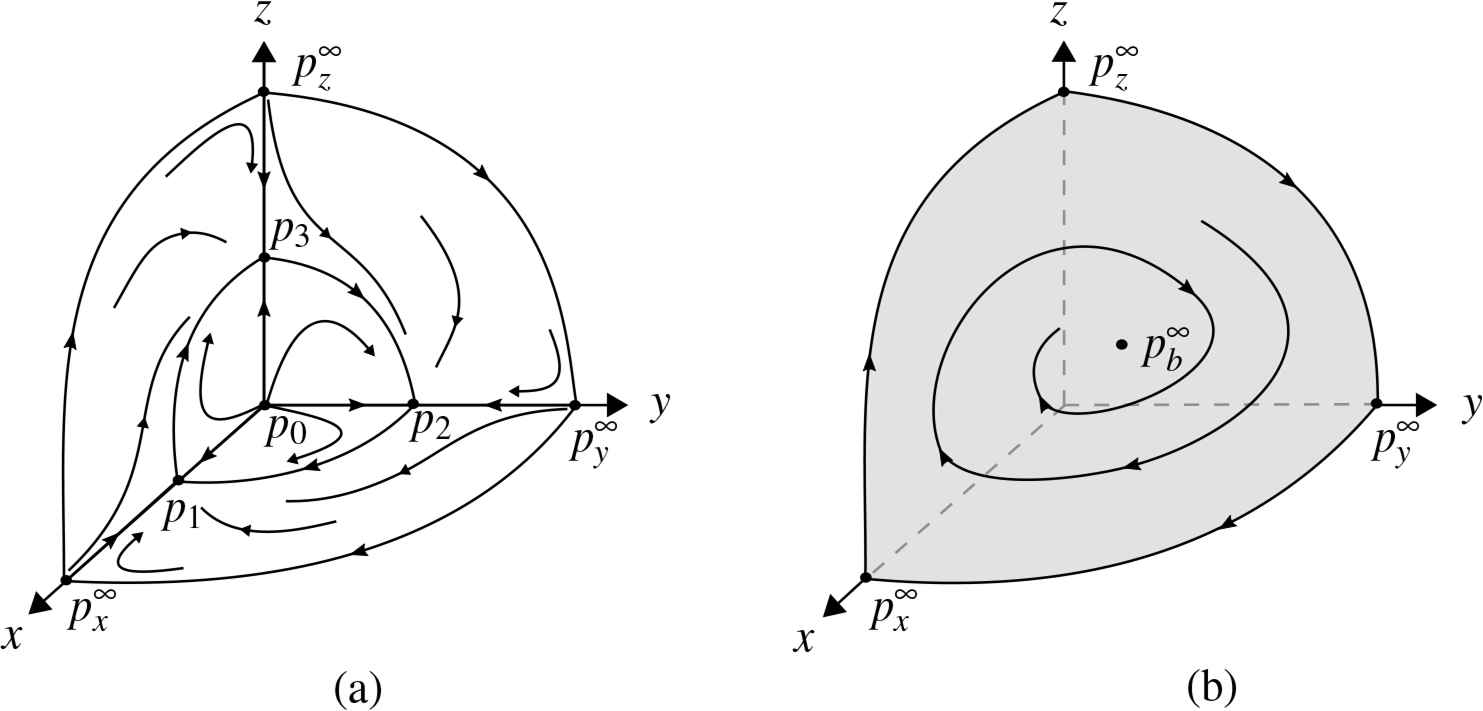
The global dynamics on the boundary of R for a + b = −1 and a ≤ −2. (a) The dynamics on xyz = 0. (b) The dynamics on R∞. Reversing the sense of all the orbits we have the global dynamics on the boundary of R for a + b = −1 and a ≥ 1.
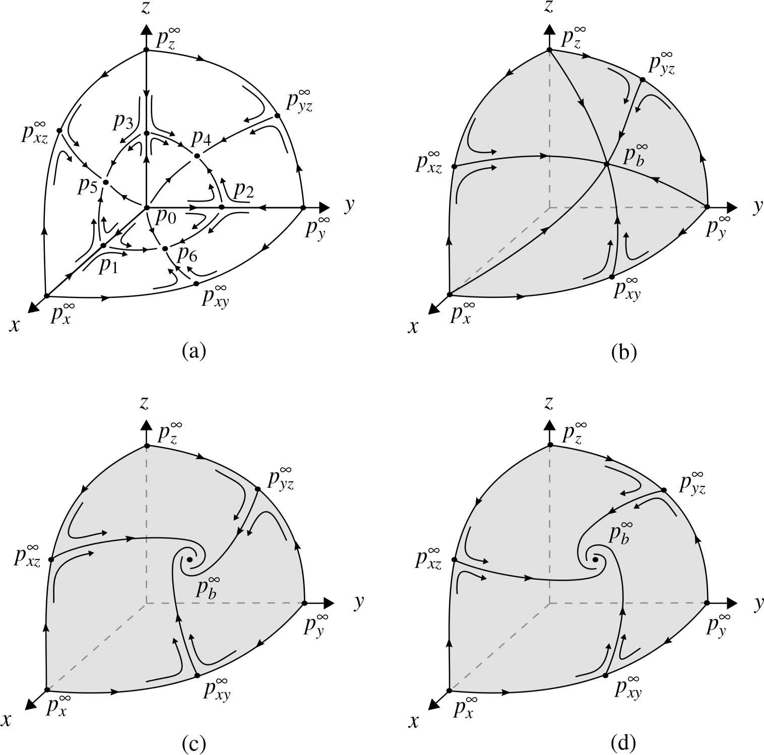
The global dynamics on the boundary of R for a + b = −1 and −2 < a < 1. (a) The dynamics on xyz = 0. The dynamics on R∞ for a = −1/2 in (b), for a ∈ (−2, −1/2) in (c), and for a ∈ (−1/2, 1) in (d).
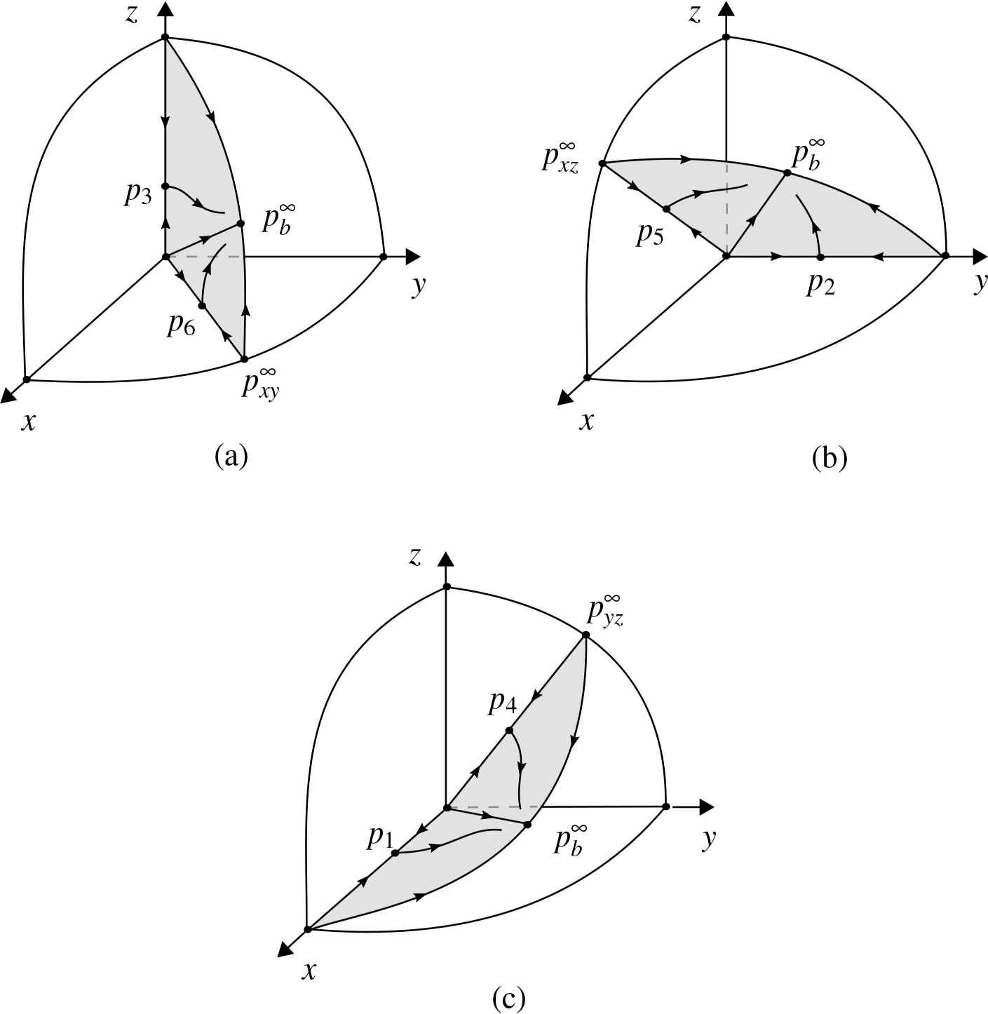
The global dynamics on R ∩ {x = y}, R ∩ {x = z} and R ∩ {y = z} respectively, when a = b = −1/2.
Let p(γ) denote the orbit γ of the vector field X associated to system (1.1) in the Poincaré compactification p(X).
Theorem 2.2.
Let γ be an orbit of system (1.1) with a + b = −1 such that p(γ) is contained in the interior of R. Then the following statements hold.
- (a)
If a ≤ −2 or a ≥ 1 then we have:
- (i)
The α-limit set of p(γ) is either the origin of ℝ3, or the heteroclinic loop connecting the singular points p1, p2 and p3, or the heteroclinic loop connecting the singular points
- (ii)
The ω-limit set of p(γ) is either
- (i)
- (b)
If −2 < a < 1 then we have:
- (i)
The α-limit set of p(γ) is one of the singular points pj for j = 0, 1... , 6 or
- (ii)
The ω-limit set of p(γ) is
- (i)
An immediate consequence of Theorem 2.2 is the following result.
Corollary 2.1.
All orbit γ of system (1.1) with a + b = −1 such that p(γ) is contained in the interior of R has their α-limit in xyz = 0 and their ω-limit in R∞.
3. Proof of Theorem 1
The following two lemmas will be useful to the proof of Theorem 1.
Lemma 3.1.
The May-Leonard differential system (1.1) with a+ b = −1 has four finite equilibrium points in the case a ≤ −2 or a ≥ 1, and has seven finite equilibrium points in the case −2 < a < 1. Moreover, the local dynamics around these equilibrium points are presented in Figures 1(a) and 2(a).
Proof.
The finite singular points of system (1.1) with a + b = −1 are the solutions of the system
Since A > 0 for a ∈ ℝ and the region of interest is R, we have:
- (i)
If a ≤ −2 or a ≥ 1 system (1.1) has only four finite equilibrium points: p0, p1, p2 and p3.
- (ii)
If −2 < a < 1 system (1.1) has the seven finite equilibrium points pj for j = 0, 1... , 6.
All these finite equilibrium points are hyperbolic if a ≠ −2,1, and consequently its local phase portrait is topologically equivalent to the phase portrait of its linear part by the Hartman–Grobman Theorem, see for instance [4].
We note that when a ∈ (−2,1) and a → 1 we have that p4 → p3, p5 → p1 and p6 → p2; while if a → −2 we have that p4 → p2, p5 → p3 and p6 → p1. This behavior of these equilibria allows to determine by continuity the local phase portraits on the boundary of R of the non-hyperbolic equilibrium points p1, p2 and p3 when a = −2 and a = 1 from the global phase portraits of the boundary of R when a ∈ (−2,1).
The linear part of system (1.1) at the equilibrium p0 is the identity matrix. Therefore it is a repelling equilibrium.
The eigenvalues of linear part at equilibrium points p1, p2 and p3 are −1, 1− a, 2+ a. Therefore when a < −2 or a > 1 these equilibria have a 2-dimensional stable manifold and an 1-dimensional unstable one; and for −2 < a < 1 these equilibria have a 2-dimensional unstable manifold and an 1-dimensional stable one.
When −2 < a < 1 the eigenvalues of linear part at equilibrium points p4, p5 and p6 are 3, −1 and (−2 + a + a2)/A. Since −2 + a + a2 < 0 for −2 < a < 1 then these equilibria have a 2-dimensional stable manifold and an 1-dimensional unstable one. Moreover, p4 (respectively p5 and p6) is an attractor restricted to the invariant boundary x = 0 (respectively y = 0 and z = 0). Now we explain in few words, what we mean by saying that the local phase portraits, for a = −2 and a = 1, can be determined by continuity. For example, if a ∈ (−2,1) then, on the plane x = 0, we have that p4 is a node and p2 is a saddle. If a tends to −2 then p4 tends to p2 and we have a saddle-node bifurcation. For a = −2 we have that p4 = p2 is a saddle-node singularity with two hyperbolic sectors in the half-plane {x = 0,y < 0} and a parabolic sector in the half-plane {x = 0,y > 0}. So, in a neighborhood of p2 contained in the half-plane {x = 0, y > 0}, the local phase portraits are the same for a = −2 or a < −2 in the non-negative octant. The same analysis can be done for the other points p1 and p3, and for the case when a tends to 1.
Lemma 3.2.
The May-Leonard differential system (1.1) with a + b = −1 has four infinite equilibrium points in the case a ≤ −2 or a ≥ 1, and has seven infinite equilibrium points in the case −2 < a < 1. Moreover, the local dynamics around these equilibrium points are presented in Figures 1(b), 2(b), 2(c) and 2(d).
Proof.
Now we shall study the infinite equilibrium points. For study the dynamics on the infinity R∞ of R we shall use the Poincaré compactification of the differential system (1.1). See appendix for details. Thus the differential system (1.1) in the local chart U1 becomes
So system (1.1), with a + b = −1 and satisfying a ≤ −2 or a ≥ 1, has two equilibrium points at infinity: (0, 0, 0) and (1, 1, 0). We call the first one
The eigenvalues of linear part at equilibrium
Now system (1.1) in the local chart U2 writes
Since the local chart U2 covers the end part of the plane x = 0 at infinity of the non-negative octant of ℝ3, we are interested only in the equilibrium points which are on z1 = 0 and z3 = 0. In this case, with a + b = −1 and satisfying a ≤ −2 or a ≥ 1, there is one equilibrium point at infinity: (0, 0, 0). We call this equilibrium
Now for a ≤ −2 or a ≥ 1 we only need to study the equilibrium point at the endpoint of positive z-half-axis, i.e. the equilibrium point at the origin of the local chart U3. We call this equilibrium point
The linear part at the equilibrium point
We have proved that the phase portrait of system (1.1) on R∞, for a + b = −1 and a ≤ −2, is the one presented in Figure 1(b). In the same figure, reversing the sense of all the orbits, we have the global dynamics on R∞, for a + b = −1 and a ≥ 1.
It remains to study the infinite equilibrium points of system (1.1) in case −2 < a < 1. In the local chart U1 the system (3.1) has four equilibrium points at infinity:
Now since we are interested only in the equilibrium points which are on z1 = 0 and z3 = 0, in the local chart U2 the system (3.2) has two equilibrium points:
In the local chart U3 we only need to study the equilibrium point
We conclude that the infinite equilibrium points of system (1.1) with a + b = −1 in case −2 < a < 1 are
We also observe that when a ∈ (−2,1) and a → 1 we have that
We will show now that does not exist a periodic orbit on R∞. For this we will need Bautin’s Theorem, which is proved in [1].
Theorem 3.1 (Bautin’s Theorem).
A quadratic polynomial differential system of the form
Lemma 3.3
There are no periodic orbits of the Poincaré compactification of the vector field associated to system (1.1) in the Poincaré compactification on R∞.
Proof.
The differential system (1.1) in the local chart U1 is given by (3.1). Making z3 = 0 to determine the dynamics on R∞ we have the system
By Bautin’s Theorem, the system (3.3) has no limit cycles. In addition, system (3.3) has only two equilibrium points: (z1, z2) = (0, 0) and (z1, z2) = (1,1). The linear part at the equilibrium (0,0) has the eigenvalues 1 − a and 2 + a, and the eigenvalues of linear part at equilibrium (1,1) are
So, using Lemmas 3.1, 3.2 and 3.3, the proof of statements (a) and (b) of Theorem 2.1 is complete.
Now since the bisectrix x = y = z is an invariant straight line for the system, it is easy to check for a = −1/2 that the global phase portrait on the invariant planes R ∩ {x = y}, R ∩ {x = z} and R ∩ {y = z} are topologically equivalents to the ones described in (a), (b) and (c) of Fig. 3 respectively. This completes the proof of Theorem 2.1.
4. Proof of Theorem 2
We say that a C1 function I(x, y, z, t) is an invariant of the polynomial differential system (1.1) if I(x(t), y(t), z(t), t) is constant, for all the values of t for which the solution (x(t), y(t), z(t)) of (1.1) is defined. When the function I is independent of the time, then it is called a first integral of differential system (1.1). Also if an invariant I(x, y, z, t) is of the form f(x, y, z)est, then it is called a Darboux invariant.
Proposition 4.1.
System (1.1), for a + b = −1, has the Darboux invariant I = I(t, x, y, z) = xyze−3t.
Proof.
It is immediate to check that
For knowing how to obtain the Darboux invariant given in Proposition 4.1 see statement (vi) of Theorem 8.7 of [5], there the theory is described for polynomial vector fields in ℝ2, but the results and the proofs extend to ℝ3.
Proposition 4.2.
Let I(x, y, z, t) = f(x, y, z)est be a Darboux invariant of system (1.1). Let p ∈ ℝ3 and φp(t) the solution of system (1.1) such that φp(0) = p. Then
Here α(p) and ω(p) denote the α-limit and ω-limit sets of p respectively, and 𝕊2 denotes the boundary of the Poincaré ball, i.e. the infinity of ℝ3.
For a proof of Proposition 4.2 see [7].
Lemma 4.1.
Let p(γ) = {φp(t) = (x(t), y(t), z(t)) : t ∈ ℝ} be the orbit of the Poincaré compactification of system (1.1), for a + b = −1, such that φp(0) = p and
Proof.
Let q ∈ ω(p). Then there exists a sequence (tn) with tn → +∞, such that φp(tn) = (x(tn), y(tn), z(tn)) → q when n → +∞. By Proposition 4.2 we know that q ∈ {(x, y, z) ∈ R : xyz = 0} ∪ R∞. Suppose that q ∉ R∞ and take ε > 0. Then there exist M > 0 and n0 ∈ ℕ such that xyz ≤ M for all
Proof.
[Proof of Theorem 2.2] Let p(γ) = {φp(t) = (x(t), y(t), z(t)) : t ∈ ℝ} be the orbit of the Poincaré compactification of system (1.1) with a+b = −1 such that φp(0) = p with p in the interior of R. We recall that all the orbits of a differential system defined on a compact set are defined for all t ∈ ℝ. By Propositions 4.1 and 4.2 the α- and ω-limit set of p(γ) is contained in boundary of R, i.e. in {(x, y, z) ∈ R : xyz = 0} ∪ R∞. Furthermore, by Proposition 4.1, I(t, x(t), y(t), z(t)) = k constant with k > 0. So
This implies that the orbit p(γ) tends to the set xyz = 0 when t → −∞. Looking at the dynamics of the flow of the compactified vector field on xyz = 0 described in Fig. 1(a) if a ≤ −2 or a ≥ 1, and in Fig. 2(a) if −2 < a < 1, we consider the following two cases.
Case 1. Suppose that a ≤ −2 or a ≥ 1. Therefore, by Theorem 2.1(a) and Fig. 1(a) we have that the α-limit set of p(γ) can be the equilibrium point p0 because the eigenvalue at p0 is 1 with multiplicity three. The equilibrium points p1, p2, p3,
Case 2. Assume that −2 < a < 1. By Theorem 2.1(a) and Fig. 2(a) we have that the singular points p0,
Now we study the ω-limit set of p(γ). In a similar way taking limit in (4.1) when t → +∞ we obtain
So by Proposition 4.2 and by Lemma 4.1 we conclude that the ω-limit set of p(γ) is contained in R∞. Looking at the dynamics of the flow of the compactified vector field on R∞ described in Fig. 1(b) if a ≤ −2 or a ≥ 1, we conclude that the ω-limit set of p(γ) is the infinite singular point
Remark 4.1.
An interesting question is: Can we say something for other values of the parameters a and b? As we have mentioned at the beginning of Section 4, both Darboux invariant and first integral are invariants to the system (1.1). Leach and Miritzis [6] obtained the following first integrals:
- (i)
- (ii)
- (iii)
The global dynamics in these cases was studied in [2].
Appendix
A. The Poincaré compactification in ℝ3
For more details on the Poincaré compactification in ℝ3 see [3]. In ℝ3 we consider the polynomial differential system
Let 𝕊3 = {y = (y1, y2, y3, y4) ∈ ℝ4 : ‖y‖ = 1} be the unit sphere in ℝ4, and
We consider the central projections
The diffeomorphisms f+ and f− define two copies of X, one Df+ ○ X in the northern hemisphere and the other Df− ○ X in the southern one. Denote by
In what follows we shall work with the orthogonal projection of the closed northern hemisphere to y4 = 0. Note that this projection is a closed ball B of radius one, whose interior is diffeomorphic to ℝ3 and whose boundary 𝕊2 corresponds to the infinity of ℝ3. The projected vector field on B is called the Poincaré compactification on the Poincaré ball B.
As 𝕊3 is a differentiable manifold, to compute the expression for p(X) we can consider the eight local charts (Ui, Fi), (Vi, Gi) where Ui = {y ∈ 𝕊3 : yi > 0} and Vi = {y ∈ 𝕊3 : yi < 0} for i = 1,2,3,4; the diffeomorphisms Fi : Ui → ℝ3 and Gi : Vi → ℝ3 for i = 1,2,3,4, are the inverses of the central projections from the origin to the tangent planes at the points (±1,0,0,0), (0,±1,0,0), (0,0,±1,0) and (0,0,0,±1), respectively. The expression of p(X) on the local chart U1 is
The expression for p(X) in U4 is
Acknowledgments
The first author is supported by FAPESP grant 2013/2454-1 and CAPES grant 88881.068462/2014-01. The second author is partially supported by the Ministerio de Economía, Industria y Competitividad, Agencia Estatal de Investigación grant MTM2016-77278-P (FEDER), the Agència de Gestió d’Ajuts Universitaris i de Recerca grant 2017SGR1617, and the H2020 European Research Council grant MSCA-RISE-2017-777911. The third author is supported by CAPES grant 99999.006888/2015-01 from the program CAPES-PDSE.
References
Cite this article
TY  - JOUR
AU  - Claudio A. Buzzi
AU  - Robson A. T. Santos
AU  - Jaume Llibre
PY  - 2020
DA  - 2020/01/27
TI  - Final evolutions of a class of May-Leonard Lotka-Volterra systems
JO  - Journal of Nonlinear Mathematical Physics
SP  - 267
EP  - 278
VL  - 27
IS  - 2
SN  - 1776-0852
UR  - https://doi.org/10.1080/14029251.2020.1700635
DO  - 10.1080/14029251.2020.1700635
ID  - Buzzi2020
ER  -