Journal of Nonlinear Mathematical Physics

Volume 27, Issue 2, January 2020, Pages 279 - 294

A generalization of the Landau-Lifschitz equation: breathers and rogue waves

Authors
Ruomeng Li, Xianguo Geng*, Bo Xue
School of Mathematics and Statistics, Zhengzhou University, 100 Kexue Road, Zhengzhou, Henan 450001, People’s Republic of China,liruomeng@zzu.edu.cn(RM Li);xggeng@zzu.edu.cn(XG Geng);xuebo@zzu.edu.cn(B Xue)
*Corresponding author (xggeng@zzu.edu.cn)
Corresponding Author
Xianguo Geng
Received 9 June 2019, Accepted 11 September 2019, Available Online 27 January 2020.
DOI
10.1080/14029251.2020.1700636How to use a DOI?
Keywords
generalized uniaxial Landau-Lifschitz equation; N-fold generalized Darboux transformation; Akhmediev breathers; solitons; rogue waves
Abstract

A generalization of the Landau-Lifschitz equation with uniaxial anisotropy is proposed, which can also reduce to the derivative nonlinear Schrödinger equation under an infinitesimal parameter. Based on the gauge transformation between Lax pairs, an N-fold generalized Darboux transformation is constructed for the generalization of the Landau-Lifschitz equation with uniaxial anisotropy. As applications of the N-fold generalized Darboux transformations, several types of exact solutions of the generalization of the Landau-Lifschitz equation with uniaxial anisotropy are obtained, including soliton solutions, Akhmediev breather solutions and rogue-wave solutions.

Copyright
© 2020 The Authors. Published by Atlantis and Taylor & Francis
Open Access
This is an open access article distributed under the CC BY-NC 4.0 license (http://creativecommons.org/licenses/by-nc/4.0/).

1. Introduction

The continuous classical Heisenberg ferromagnet equation (the Heisenberg equation for short) can be written as either

iqtwqxx+wxxq=0,|q|2+w2=1,(1.1)
or
Qt+Q×Qxx=0,QQ=1,(1.2)
where q is a complex potential, w is a real potential, Q = (Req, Imq, w)T is a column vector, the symbols × and · denote the cross and the dot product, respectively. In Ref. [38], the inverse scattering method was applied to the Heisenberg equation. The gauge transformations between the Heisenberg equation (1.2) and the focusing or the defocusing nonlinear Schrödinger equations are found [28, 43]. An effective approach [11] is developed to obtain the generation of closed-form solitons solution of the Heisenberg equation (1.2). In Ref. [2], the higher-order soliton solutions of the Heisenberg equation (1.2) are constructed by using the Darboux transformation (see Refs. [13, 15, 17, 18, 22, 26, 27, 29, 32, 36, 39, 40, 44, 45]). The Heisenberg equation (1.2) is the isotropic case of the Landau-Lifschitz (LL) equation,
Qt+Q×Qxx+Q×(JQ)=0,QQ=1,(1.3)
where J = diag{J1, J2, J3} is a real diagonal matrix, J1J2J3, which can be reduced to the sine-Gordon equation and the nonlinear Schrödinger equation [12]. The Cauchy problem for the LL equation (1.3) is studied by using the inverse transform method, and the Cauchy problem is also changed into the matrix Riemann problem on a torus and a certain Fredholm integral equation, from which an exact N-soliton solution is constructed [30, 33, 34]. When J1 = J2 or J2 = J3, the LL equation is called an LL equation with uniaxial anisotropy (a uniaxial LL equation for short). Please see Refs. [3,4] and the references therein for more information on the names of this equation. Particularly, when J = diag{0,0,4β}, the LL equation (1.3) can be rewritten as
iqtwqxx+wxxq+4βwq=0,|q|2+w2=1,β.(1.4)

In Ref. [20], a Darboux transformation of the LL equation (1.4) was constructed and its various exact solutions were obtained. The Heisenberg equation (1.2) is also called the isotropy LL equation [2, 20, 37].

In this paper, we propose a generalized uniaxial LL equation (a guLL equation for short),

iqtwqxx+wxxq+2iα(w2q)x+4βwq=0,|q|2+w2=1,α,β,(1.5)
or equivalently
Qt+Q×Qxx+4βQ×(J^Q)+α{Q×[Q×(J^Q)]J^Q}x=0,(1.6)
where Ĵ= diag(0,0,1). Apparently, equation (1.5) can be reduced to the uniaxial LL equation (1.4) and the Heisenberg equation (1.1) when α = 0 and α = β = 0, respectively. Let ε ∈ ℝ be a small parameter and q = εu, α = ε−2 and β = 0. Then (1.5) can be rewritten as
iut1ε2|u|2uxx+(1ε2|u|2)xxu2i(|u|2u)x=0,(1.7)
which turns out the derivative nonlinear Schrödinger equation
iutuxx2i(|u|2u)x=0,(1.8)
when ε → 0. Therefore, (1.5) is closely related to the derivative nonlinear Schrödinger equation (1.8).

Rogue waves are giant wave events in nonlinear deep water gravity waves that rise to surprising heights above the background wave field. Holes are deep troughs which occur before and/or after the largest crests [31]. Rogue periodic waves [7,8], rouge waves [5,6] and other exact solutions [35] are always interesting issues. Solitons and breathers are also important nonlinear phenomena that attract much attention. Our main aim in this paper is to construct N-fold Darboux transformations, by which soliton solutions, breather solutions and rogue-hole solutions of the guLL equation (1.5) are obtained. Some special limits of N-fold Darboux transformations are called generalized Darboux transformations [19], by which rogue wave solutions of the corresponding integrable nonlinear equation can be obtained. However, it is difficult to calculate the limits of N-fold Darboux transformations. To solve this problem, we give a formula for generalized Darboux transformations without taking limits. Because classical and generalized Darboux transformations are given by the same formula (2.33) in this paper, classical and generalized Darboux transformations are both called N-fold Darboux transformations for simplicity.

The major innovations of the present paper include the following aspects. First, we propose a generalized uniaxial anisotropy Landau-Lifschitz equation (1.5), which contains two arbitrary constants α, β ∈ ℝ. Second, we give exact formulas for N-fold Darboux transformations without taking limits. Avoiding limits can greatly reduce computational complexity, especially when the seed solution is not trivial or when N is large. Third, as applications of the obtained Darboux transformations, several nonlinear phenomena (e.g., solitons, breathers and rogue holes) are revealed.

The outline of this paper is as follows. In Section 2, we present a Lax pair for the guLL equation and then construct its N-fold generalized Darboux transformations with the help of gauge transformations between Lax pairs. In Section 3, as applications of the multi-fold generalized Darboux transformations, we obtain various explicit solutions for the generalization of the guLL equation, including soliton solutions, Akhmediev breather solutions and rogue-hole solutions.

2. Lax pair and Darboux transformations

The spectral and auxiliary problems associated with the guLL equation (1.5) read

Φx(λ)=U(λ)Φ(λ),Φt(λ)=V(λ)Φ(λ),(2.1)
where Φ(λ) = Φ(x, t, λ) is a 2 × 1 vector eigenfunction, λ ∈ ℂ is a constant spectral parameter, and
U(λ)=(iλw(λζ1)q(λζ2)q*iλw),V(λ)=(iλb+2i(λζ1)(λζ2)w(λζ1)(a+2λ)q(λζ2)(a*+2λq*)iλb2i(λζ1)(λζ2)w),a=i(wqxqwx)(ζ1+ζ2)w2q,b=Im(q*qx)+(ζ1+ζ2)(2ww3),(2.2)
where ζ1 and ζ2 are the two roots of ζ2 − 2αζ + β = 0. Here we assume that ζ1ζ2 ∈ ℝ and ζ1 +ζ2 ∈ ℝ, which means: (i) if ζ1 ∈ ℝ, then ζ2 ∈ ℝ; otherwise (ii) if ζ1 ∈ ℂ \ ℝ, then ζ2=ζ1*.

Suppose that Ψ(λ) = Ψ(x, t, λ) is the fundamental solution matrix of (2.1) with the initial condition

Ψ(0,0,λ)=I2,(2.3)
and expand Ψ(λ + ε) into the Taylor series,
Ψ(λ+ε)=j=01j!Ψ(j)(λ)εj=10!Ψ(λ)+11!Ψ˙(λ)ε+12!Ψ¨(λ)ε2+13!Ψ(λ)ε3+,(2.4)
where Ψ(j)(λ)=jλjΨ(λ), Ψ˙(λ)=Ψ(1)(λ), Ψ¨(λ)=Ψ(2)(λ) and Ψ(λ)=Ψ(3)(λ). Denote
U˙=λU(λ),V˙(λ)=λV(λ),V¨=2λ2V(λ),(2.5)
where U˙(λ) and V¨(λ) are written as U˙ and V¨, because they are independent of λ. Taking the derivatives of (2.1) with respect to λ to the jth order we have
Ψ˙x(λ)=U(λ)Ψ˙(λ)+U˙Ψ(λ),Ψ˙t(λ)=V(λ)Ψ˙(λ)+V˙(λ)Ψ(λ),Ψx(j)(λ)=U(λ)Ψ(j)(λ)+jU˙Ψ(j1)(λ),Ψt(j)(λ)=V(λ)Ψ(j)(λ)+jV˙(λ)Ψ(j1)(λ)+12j(j1)V¨Ψ(j2)(λ),(j2).(2.6)

Substituting

U(λ)=Ψ(λ)[Ψ(λ)1]x,V(λ)=Ψ(λ)[Ψ(λ)1]t(2.7)
into (2.6), we find
[Ψ(λ)1Ψ˙(λ)]x=Ψ(λ)1U˙Ψ(λ),[Ψ(λ)1Ψ˙(λ)]t=Ψ(λ)1V˙(λ)Ψ(λ),[Ψ(λ)1Ψ(j)(λ)]x=jΨ(λ)1U˙Ψ(j)(λ),[Ψ(λ)1Ψ˙(j)(λ)]t=jΨ(λ)1V˙Ψ(j1)(λ)+12j(j1)Ψ(λ)1V¨Ψ(j2)(λ)(j2).(2.8)

Using (2.3) we have

Ψ˙(x,t,λ)=(0,0)(x,t)Ψ(x,t,λ)Ψ(x^,t^,λ)1[U˙(x^,t^)dx^+V˙(x^,t^,λ)dt^]Ψ(x^,t^,λ),Ψ(j)(x,t,λ)=(0,0)(x,t)Ψ(x,t,λ)Ψ(x^,t^,λ)1[jU˙(x^,t^)dx^+jV˙(x^,t^,λ)dt^+12j(j1)V¨(x^,t^,λ)dt^]Ψ(j1)(x^,t^,λ)(j2).(2.9)

In terms of Ψ(λ), a general solution Φ(λ) of the Lax pair (2.1) can be given by

Φ(x,t,λ)=Ψ(x,t,λ)Y(λ),(2.10)
where Y(λ) = Φ(0, 0, λ) denotes an intial condition. Resorting to
Φ(j)(λ)=jλjΦ(λ)=k=0j(jk)Ψ(jk)(λ)Y(k)(λ),(2.11)
we can give Φ(j)(λ) in terms of {Ψ (0)(λ),...,Ψ(j)(λ)}.

Suppose λ1,...,λK ∈ ℂ \ ℝ, (λjλk if jk), and N1,...,NK ∈ 𝕑+ are fixed. Set N = N1 + ··· + NK, and denote

Φk=Φ(λk),Φk(j)=Φ(j)(λk),(1kK,0jNk1).(2.12)

Remark 2.1.

From (2.11) it is apparent that

Φk(j)=l=0j(jl)Ψ(jl)(λk)Y(l)(λk),(1kK,0jNk).(2.13)

The quantities Ψ(j)(λk) can be obtained from two approaches. First, one can solve the Lax pair (2.1) at λ = λk + ε, and then calclculate the derivatives jεj|ε=0Ψ(λk+ε). However, when the seed solution is not trivial, even though it is easy to obtain Ψ(λk), it is usually difficult or tedious to obatin the exact expression of Ψ(λk + ε), however small ε is. Therefore, we develop a second approach, i.e., the equations (2.9) and (2.11). In this approach, the spectral constant λk is fixed. The derivatives with resect to λ are replaced with integrals with resect to (x, t). In practice, we find the integrals in (2.9) are always easy to calculate with the support of some mathematical software, like <monospace>Mathematica</monospace>. The quantites Y(j)(λk) denotes some arbitrary constants, because Y(λ) is the initial condition of Φ(x, t, λ) that can be chosen freely.

Now we construct an N-fold generalized Darboux transformation directly in terms of N quantities

{Φk(j)|1kK,0jNk}(2.14)
without taking limits. In order to derive a Darboux transformation, we have to find a Darboux matrix 𝒯(λ) and two new potentials q˜ and w˜ such that Φ˜(λ)=𝒥(λ)Φ(λ) satisfies the new Lax pair
Φ˜x(λ)=U˜(λ)Φ˜(λ),Φ˜t(λ)=V˜(λ)Φ˜(λ),(2.15)
where U˜(λ)=U(λ)|q=q˜,w=w˜ and V˜(λ)=V(λ)|q=q˜,w=w˜. A direct calculation shows that 𝒯(λ) satisfies
U˜(λ)𝒥(λ)=𝒥x(λ)+𝒥(λ)U(λ),V˜(λ)𝒥(λ)=𝒥t(λ)+𝒥(λ)V(λ).(2.16)

To construct an N-fold generalized Darboux transformation, we assume that 𝒯(λ) is a suitable polynomial of degree N. For the sake of simplicity, we first consider the one-fold case. In this case, we write q˜, w˜ and 𝒯(λ) as q^, ŵ and T (λ), respectively, to emphasize that N = 1.

Theorem 2.1.

Suppose that (q, w) is a known solution of the guLL equation (1.5), and fix λ1 ∈ ℂ\ℝ. Assume that Φ1 = Φ(λ1) = (ϕ1, ψ1)T is a solution of the Lax pair (2.1) when λ = λ1 and ϕ1 ≠ 0. Suppose r and s are defined by

r=1+(λ1ζ1)(λ1ζ2)|ρ1|2λ1+λ1*(λ1ζ1)(λ1ζ2)|ρ1|2,s=(λ1λ1*)ρ1*λ1+λ1*(λ1ζ1)(λ1ζ2)|ρ1|2,(2.17)
where ρ1=(λ1ζ2)1ψ1φ11. Then (q^,w^) determined by the Darboux transformation
q^=msm*s*q*mxζ1ζ2m*s*,w^=w+imxζ1ζ2mr(2.18)
is a new solution of the guLL equation (1.5), and
T(λ)=(m(1+λr)(λζ1)ms(λζ2)m*s*m*(1+λr*))(2.19)
is the corresponding Darboux matrix, where
m={[(1+ζ1r)ζ2(1+ζ2r)ζ1]1/(ζ1ζ2),ifα2β,11+αreαr1+αr,ifα2β.(2.20)

Moreover, Φ^(λ)=T(λ)Φ(λ) satisfies the new Lax pair

Φ^x=U^Φ,Φ^t=V^Φ^,U^=U|q=q^,w=w^,V^=V|q=q^,w=w^.(2.21)

Proof.

We first prove that (q^,w^) is a new solution of the guLL equation (1.5) by proving that T(λ) satisfies (2.16). For notation convenience, we denote

D(λ)=(D1(λ)(λζ1)D2(λ)(λζ2)D2(λ*)*D2(λ*)*)=U^(λ)T(λ)Tx(λ)T(λ)U(λ),Δ(λ)=(Δ1(λ)(λζ1)Δ2(λ)(λζ2)Δ2(λ*)*Δ1(λ*)*)=V^(λ)T(λ)Tt(λ)T(λ)V(λ),(2.22)
and aim at showing D(λ) ≡ 0 and Δ(λ) ≡ 0.

When (w^,q^) are defined by (2.18), it is easy to see that D1(λ) is a linear polynomial in λ and D1(0) = 0. When (2.20) holds, we have

mxm=ζ1ζ2rrx1+(ζ1+ζ2)r+ζ1ζ2r2,(2.23)
which implies D1(λ) ≡ 0. From T(λ11 = 0 we can derive
D(λ1)Φ1=U^(λ1)T(λ1)Φ1T1,xΦ1T(λ1)U(λ1)Φ1=(T1Φ1)x=0.(2.24)

Noting that D2(λ) is linear polynomials in λ, we finally arrive at D2(λ) ≡ 0, and thus D(λ) ≡ 0.

By using D(λ) ≡ 0 and (2.20), we have

mtm=ζ1ζ2rrt1+(ζ1+ζ2)r+ζ1ζ2r2.(2.25)

A straightforward calculation shows that Δ1(λ) and Δ2(λ) can written as

Δ1(λ)={[1+(ζ1+ζ2)r]λ+ζ1ζ2r}δ1,Δ2(λ)=δ2,(2.26)
where δ1 and δ2 are functions of (x, t). In view of
Δ(λ1)Φ1=V^(λ1)T(λ1)Φ1T1,tΦ1T(λ)V(λ1)Φ1=(T1Φ1)t=0,(2.27)
we obtain Δ1(λ) ≡ Δ2(λ) ≡ 0, which means Δ(λ) ≡ 0.

Since D(λ) ≡ Δ(λ) ≡ 0, (q^,w^) must be a new solution of the guLL equation (1.5). Note that the coefficients of λ2 in D(λ) = 0 implies

(iw^q^q^*iw^)(mrmsm*s*m*r*)=(mrmsm*s*m*r*)(iwqq*iw),(2.28)
and hence |q^|2+w^2=1 and ŵ = ŵ *.

Now we make full use of the N quantities (2.14) to construct and N-fold Darboux transformation. Note, how to obtain the quantites (2.14) is well introduced in Remark 2.1.

Theorem 2.2.

Suppose (q, w) is a known solution of the guLL equation (1.5). Fix λ1,...,λK ∈ ℂ\ℝ, (λjλk if jk) and choose N1,...,NK ∈ 𝕑+. Denote N = N1 + ··· + NK. Suppose Φk and Φk(j) are defined by (2.9), (2.11) and (2.12). Suppose 𝒯(λ) is a polynomial in λ of degree N,

𝒥(λ)=(M[1+λR(λ)](λζ1)MS(λ)(λζ2)M*S(λ*)*M*[1+λR(λ*)*]),(2.29)
where R(λ) = R(x, t, λ) and S(λ) = S(x, t, λ) are polynomials in λ of degree N − 1,
R(λ)=j=1Nλj1Rj,S(λ)=j=1Nλj1Sj,(2.30)
and M = M(x, t) is given by the values R(ζ1) = R(x, t, ζ1) and R(ζ2) = R(x, t, ζ2),
M={{[1+ζ1R(ζ1)]ζ2[1+ζ2R(ζ2)]ζ1}1/(ζ1ζ2),ifα2β,11+αR(α)exp[αR(α)+α2R(α)1+αR(α)],ifα2=β.(2.31)

Suppose 𝒯(λ) satisfies the equations

l=0j(jl)𝒥(jl)(λk)Φk(l)=0,(1kK,0jNk),(2.32)
where 𝒥(j)(λ)=jλj𝒥(λ). Then (i) Rj and Sj, (1 ≤ jN), are uniquely determined by (2.32); (ii) (q˜,w˜) determined by the N-fold Darboux transformation
q˜=M(RN2q+SN2q*2iRNSNw)M*(|RN|2+|SN|2),w˜=iRNSN*q+iRN*SNq*+(|RN|2|SN|2)w|RN|2+|SN|2,(2.33)
is a new solution of the guLL equation (1.5); and (iii) the corresponding Darboux matrix is 𝒯(λ). Moreover, Rj and Sj are given explicitly in (2.46) for convenience of application because the their expressions are very long.

Proof.

Denote

(λ^1,,λ^N)=(λ1,,λ1)N1,,(λK,,λK)NK,(2.34)
or equivalently
λ^1==λ^N1=λ1,λ^N1+1==λ^N1+N2=λ2,λ^(N1++NK1)+1==λ^(N1++NK1)+NK=λK.(2.35)

Then we introduce N iterated one-fold Darboux transformations T1(λ),...,TN(λ) recursively by

Tk(λ)=(mk(1+λrk)(λζ1)mksk(λζ2)mk*sk*mk*(1+λrk*)),(1kN),(2.36)
and
Tk(λ^k)Fk(λ^k)=0,mk={[(1+ζ1rk)ζ2(1+ζ2rk)ζ1]1/(ζ1ζ2),ifα2β,11+αrkeαrk1+αrk,ifα2=β.(2.37)
where F1(λ) = Φ(λ) and
Fk+1(λ)=1λλ^kTk(λ)Fk(λ)=1λλ^k[Tk(λ)Fk(λ)Tk(λ^k)Fk(λ^k)],(1kN).(2.38)

Denote 𝒥^(λ)=TN(λ)T1(λ). Then we can calculate

𝒥^(λ)Φ(λ)=TN(λ)T1(λ)F1(λ)=(λλ^1)TN(λ)T2(λ)F2(λ)=(λλ^1)(λλ^N1)TN(λ)FN(λ)=(λλ^1)(λλ^N)FN+1(λ)=(λλ1)N1(λλK)NkFN+1(λ),(2.39)
and hence
l=0j(jl)𝒥^(jl)(λk)Φk,l=jλj|λ=λk𝒥^(λ)Φ(λ)=0,(1kK,0jNk1).(2.40)

Some further but easy calculations show that 𝒥^(λ) satisfies the symmetric relation in (2.29) and (2.31). This means that 𝒯(λ) and 𝒥^(λ) satisfy the same symmetric relations and the same equations. In other words, 𝒥(λ)𝒥^(λ). Since 𝒯(λ) = TN(λ)···T1(λ), 𝒯(λ) itself is an N-fold generalized Darboux matrix. Finally, comparing the coefficients of λN+1 in Ũ(λ)𝒯(λ) = 𝒯x(λ) + 𝒯(λ)U(λ) we get (2.33).

At the end of this section, we introduce some notations to give neat formulas for RN and SN. Denote

gj(λ)=λjφ(λ),hj(λ)=(λjζ1λj1)ψ(λ),g^j(λ)=λjψ(λ*)*,h^j(λ)=(λjζ2*λj1)φ(λ*)*.(2.41)

Then (2.32) can be written as

jλj|λ=λj{φ(λ)+[R1g1(λ)++RNgN(λ)]+[S1h1(λ)++SNhN(λ)]}=0,jλj|λ=λj*{ψ(λ*)*[S1h^1(λ)++SNh^N(λ)]+[R1g^1(λ)++RNg^N(λ)]}=0,(1kK,0jNk1),(2.42)
or more compactly as
B+XA=0,(2.43)
where
X=(R1,,RN,S1,,SN),B=(B1,,BK,B^1,,B^K),Bk=(φk(0),,φk(Nk1)),B^k=((ψk(0))*,,(ψk(Nk1))*),A=(A1,,AK,A^1,,A^K),Ak=(g1(0)(λk)g1(Nk1)(λk)gN(0)(λk)gN(Nk1)(λk)h1(0)(λk)h1(Nk1)(λk)hN(0)(λk)hN(Nk1)(λk)),A^k=(g^1(0)(λk*)g^1(Nk1)(λk*)g^N(0)(λk*)g^N(Nk1)(λk*)h^1(0)(λk*)h^1(Nk1)(λk*)h^N(0)(λk*)h^N(Nk1)(λk*)).(2.44)

Noting that gl(j)(λk), hl(j)(λk), g^l(j)(λk*) and h^l(j)(λk*) are linear combinations of φk(j) and ψk(j), where

(φk(j),ψk(j))T=Φk(j)=Φ(j)(λk),(1kK,0jNk1).(2.45)
we obtain by Cramer’s rule that
Rj=detEjdetA,Sj=detEN+jdetA,(1jN),(2.46)
where Ej is obtained from A by replacing its jth row with B, (1 ≤ j ≤ 2N).

3. Exact solutions

In this section, we construct some exact solutions of the guLL equation by using the Darboux transformations. For the sake of convenience, we consider only the special case of guLL equation (1.5) when α = β = 1 (ζ1 = ζ2 = 1):

iqtwqxx+wxxq+2i(w2q)x+4wq=0,|q|2+w2=1.(3.1)

In this case, the relation (2.31) is reduced to

M=(1+j=1NRj)1exp[j=1NjRj(1+j=1NRj)1].(3.2)

Our aim is to find the typical phenomena: solitons, rogue waves or rogue holes and Akhmediev breathers. To this end, we study two seed solutions in the following two subsections.

3.1. Seed solution 1

The first seed solution of guLL equation (3.1) is taken as

q=0,w=1.(3.3)

Then the N-fold Darboux transformation (2.33) is reduced to

q˜=2iMRNSNM*(|RN|2+|SN|2),w˜=|RN|2|SN|2|RN|2+|SN|2.(3.4)

Substituting (3.3) into Lax pair (2.1), we obtain its general solution

Φ(λ)=(f1(λ)ei[2(λ2λ+1)t+λx],f2(λ)ei[2(λ2λ+1)t+λx])T,(3.5)
where f1(λ) and f2(λ) are constants of integration. In the following, we derive some exact solutions of guLL equation (3.1) by using N-fold Darboux transformations in Theorem 2.2.

Example 3.1.

Choosing K = 1, N = N1 = 1, λ1 = ξ1 + 1, and f1(λ1) = f2(λ1) = 1, (3.5) is reduced to

Φ1=Φ(λ1)=(e12(θ1+iω1),e12(θ1+iω1))T,(3.6)
where θ1 = 4η1(2ξ1 − 1)t + 2η1x and ω1=4t(η12ξ12+ξ11)2ξ1x. Based on (2.46) and (3.2), we arrive at a one-soliton solution of guLL equation (3.1)
q˜=2η1(iη1tanhθ1+ξ11)sechθ1η12+(ξ11)2exp[2iη1tanhθ1η12+(ξ11)2iω1],w˜=12η12sech2θ1η12+(ξ11)2.(3.7)

From

|q˜|=1(12η12sech2θ1η12+(ξ11)2)2,w˜=12η12sech2θ1η12+(ξ11)2,(3.8)
we can see that |q˜| and w˜ are traveling waves. When ξ1=η1=12, the solution is illustrated in Fig. 1. Please note, only |q˜| and w˜ are stationary, arg q˜ depends on t.
Fig. 1.

A stationary solution (K = 1, N1 = N = 1, λ1=12+i2)

Example 3.2.

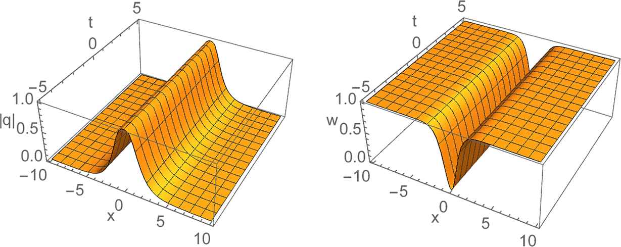
Let K = 2, N1 = N2 = 1, N = 2, and λ1 = ξ1 + 1 and λ2 = ξ2 + 2. Choose f1(λ1) = f1(λ2) = f2(λ1) = f2(λ2) = 1. Then we obtain from (3.5) that

Φ1=Φ(λ1)=(e12(θj+iωj),e12(θj+iωj))T,(1j2),(3.9)
where θj = 4ηj(2ξj − 1)t + 2ηjx and ωj=4t(ηj2ξj2+ξj1)2ξjx. Resorting to the formulas (2.44), (2.46), (2.31) and (3.4) we can obtain a two-fold Darboux transformation (q˜,w˜). The new solution (q˜,w˜) has different properties when the constants ξ1, ξ2, η1 and η2 vary.
  • Case 1: when ξ1ξ2, the new solution (q˜,w˜) is a two-soliton (see Fig. 2).

  • Case 2: when ξ1 = ξ2 and η1η2, the new solution (q˜,w˜) is a general breather (see Fig. 3).

  • Case 3: especially, when ξ1=ξ2=12 and η1η2, the new solution (q˜,w˜) is an Akhmediev breather, and the periodic in the t-direction is 12π(η12η22)1. As η2η1, the limits of q˜ and w˜ exists, e.g.,

limη1,η21/2q˜=2(8it2+4t+2ix2+2x+sinh2x)[2i(2t+x)sinhx+2(2t+xi)coshx](8t2+2x2+cosh2x+1)2×exp(4i(4t+sinh2x)8t2+2x2+cosh2x+1+2it+ix),limη1,η21/2w˜={4(8t2+2x1+1)cosh2x+8[16t4+t2(8x2+4)+8tx+x4+x2]+16(2t+x)sinh2x+cosh4x5}{2(8t2+2x2+cosh2x+1)2}1,(3.10)
Fig. 2.

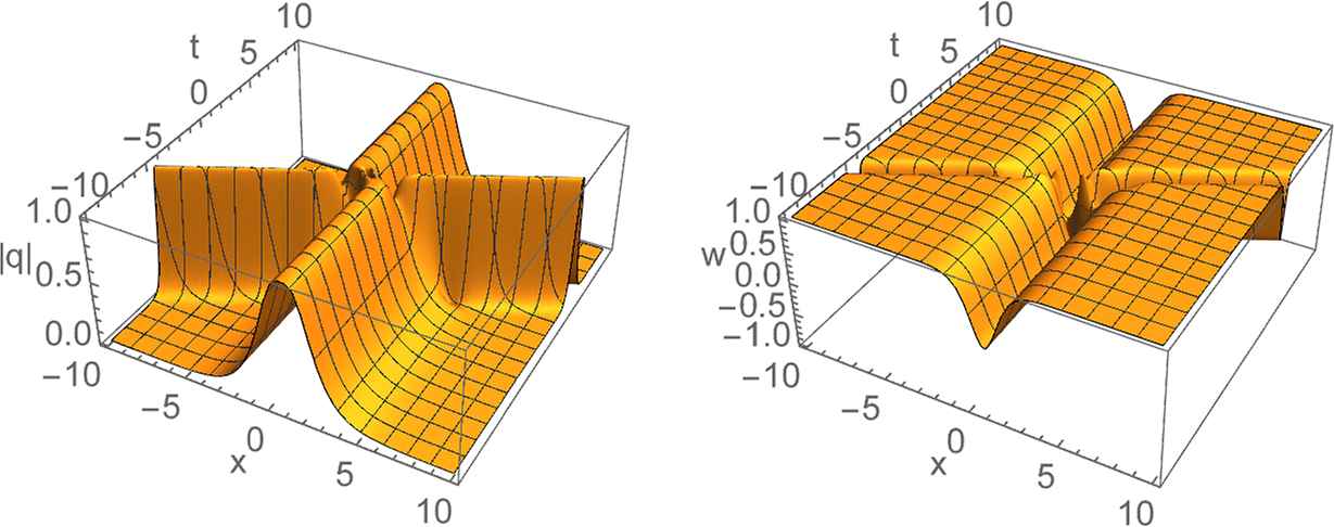
A two-soliton solution (K = 2, N1 = N2 = 1, N = 2, λ1=12+i2, λ2 = i)

Fig. 3.

An Akhmediev breather solution (K = 2, N1 = N2 = 1, N = 2, λ1=12+i2, λ2=12+i)

which is a solution (see Fig. 4) of guLL equation (3.1).
Fig. 4.

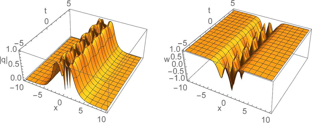
An aperiodic solution (K = 1, N1 = N = 2, λ1=12+i2)

Because taking limits always means a lot of calculations, we give an example to reduce the calculations.

Example 3.3.

Let K = 1, N = N1 = 2 and λ1 = ξ1 + 1. Choose f1(λ1) = f2(λ1) = 1 and f′1(λ1) = f′2(λ1) = 0. We have from (3.5) that

Φ1=Φ(λ1)=(e12(θ1+iω1),e12(θ1+iω1))T,Φ1(1)=Φ(1)(λ1)=[ix+it(4λ12)](e12(θ1+iω1),e12(θ1+iω1))T,(3.11)
where θ1 = 4η1(2ξ1 − 1)t + 2η1x and ω1=4t(η12ξ12+ξ11)2ξ1x. Finally, by using (2.44), (3.2) and (2.33), we can obtain a generalized Darboux transformation. Especially, when ξ1=η1=12, we arrive at the same result (3.10) without taking limits. Even though the results are the same as the limits of Case 3 in Example 3.2, the computational complexity is reduced by much. The computational complexity is usually a key issue whether an exact solution can be obtained. When K and N1,...,NK are larger, or when the seed solution is more complicated, the reduced computational complexity is more considerable.

3.2. Seed Solution 2

The second seed solution of guLL equation (3.1) is

q=e2ix,w=0.(3.12)

And the N-fold Darboux transformation (2.33) is reduced to

q˜=M(RN2e2ix+SN2e2ix)M*(|RN|2+|SN|2),w˜=iRNSN*Me2ix+iRN*SNe2ixM*(|RN|2+|SN|2).(3.13)

In the following, we construct some explicit rouge-wave solutions.

Example 3.4.

Let K = 1, N = N1 = 1 and λ1 = 1 + i. Then the Lax pair (2.1) has a solution

Φ1=Φ(λ1)=([(44i)t2ix+1]eix,[(44i)t2ix1]eix)T.(3.14)

By using (2.44), (2.31) and (2.33), we have

q˜=1024t4+512t3(2x+i)+64t2(8x2+8ix1)+16t(2x+i)3+(2x+i)4(32t2+16tx+4x2+1)2×exp(2i(32t2x+8t(2x2+1)+4x3+x)32t2+16tx+4x2+1),w˜=64t(2t+x)(32t2+16tx+4x2+1)2.(3.15)

Because

|q˜|=1[64t(2t+x)(32t2+16tx+4x2+1)2]2(3.16)
is zero at four points,
(x,t)=±(0,142),(x,t)=±(12,142),(3.17)
and |q˜|1 as max{|x|, |t|} → +∞, q˜ has four holes (see Fig. 5, where the figure of q˜ is presented upside-down for clarity).
Fig. 5.

A rouge-hole solution (K = 1, N1 = N = 1, λ1 = 1 + i). The left figure is upside-down.
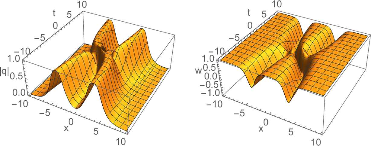
Example 3.5

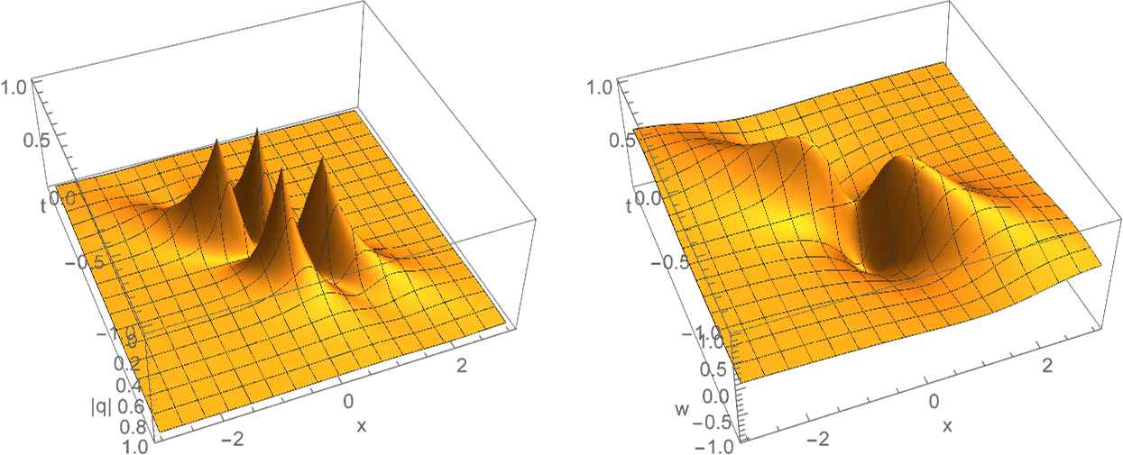
Choose K = 1, N = N1 = 2 and λ1 = 1 + i. Then the Lax pair (2.1) has a solution

Φ1=Φ(λ1)=([(44i)t2ix+1]eix,[(44i)t2ix1]eix)T,(3.18)
which together with (2.9) implies Φ1(1)=Φ(1)(λ1)
Φ1(1)=(eix{(32232i3)t3[16it2(44i)t+1]x+8t2[i+(4+4i)t]x2(2+6i)t23x3},eix{(32332i3)t3[16it2+(44i)t+1]x8t2+[i(4+4i)t]x2(2+6i)t23x3})T+f1(eix[(22i)tix+1],eix[(22i)tix])T+f2(eix[(2+2i)t+ix],eix[(22i)t+ix+1])T,(3.19)
where f1 and f2 are two constants of integration. By using (2.44), (2.31) and (2.33), we can obtain a two-fold Darboux transformation. But because the results are too tedious to write down, we only present a graphical illustration for the solution when f1 = 0, f2 = 20 in Fig. 6 (the figure of q˜ is presented upside-down for clarity).
Fig. 6.

A rouge-hole solution with more holes (K = 1, N1 = N = 1, λ1 = 1 + i). The left figure is upside-down.

Remark 3.1.

All the above explicit solutions have been verified by using Mathematica.

4. Conclusions and discussions

In this paper, a generalization of the uniaxial anisotropic Landau-Lifschitz equation is proposed. Based on the gauge transformation between Lax pairs, an N-fold generalized Darboux transformation is constructed. As applications of these Darboux transformation, several examples of exact solutions, including breather solutions and rogue-wave solutions, are given. The Landau-Lifschitz equation is important in the fields of both physics and mathematics. The generalization of the uni-axial anisotropic Landau-Lifschitz equation deserves further study.

Acknowledgments

This work is supported by National Natural Science Foundation of China (Grant Nos. 11871440, 11931017 and 11971442).

References

[2]D.F. Bian, B.L. Guo, and L.M. Ling, High-order soliton solution of Landau-Lifshitz equation, Stud. Appl. Math, Vol. 134, 2015, pp. 181-214.
[4]A.E. Borovik and S.I. Kulinich, Integration of the nonlinear dynamics of a uniaxial ferromagnet by the method of the inverse scattering problem, JETP Lett, Vol. 39, 1984, pp. 384-389.
[5]H.N. Chan and K.W. Chow, Rogue waves for an alternative system of coupled Hirota equations: structural robustness and modulation instabilities, Stud. Appl. Math, Vol. 139, 2017, pp. 78-103.
[18]C.H. Gu, H.S. Hu, and Z.X. Zhou, Darboux transformations in integrable systems: Theory and their applications to geometry, Springer, Dordrecht, 2005.
[29]V.B. Matveev and M.A. Salle, Darboux Transformations and Solitons, Springer Berlin Heidelberg, Berlin, 1991.
[35]U. Saleem and M. Hassan, Darboux transformation and exact multisolitons of ℂPN nonlinear sigma model, J. Math. Anal. Appl, Vol. 447, 2017, pp. 1080-1101.
[41]J. Xu and E.G. Fan, Initial-boundary value problem for integrable nonlinear evolution equation with 3 × 3 Lax pairs on the interval, Stud. Appl. Math, Vol. 136, 2016, pp. 321-354.
Journal
Journal of Nonlinear Mathematical Physics
Volume-Issue
27 - 2
Pages
279 - 294
Publication Date
2020/01/27
ISSN (Online)
1776-0852
ISSN (Print)
1402-9251
DOI
10.1080/14029251.2020.1700636How to use a DOI?
Copyright
© 2020 The Authors. Published by Atlantis and Taylor & Francis
Open Access
This is an open access article distributed under the CC BY-NC 4.0 license (http://creativecommons.org/licenses/by-nc/4.0/).

Cite this article

TY  - JOUR
AU  - Ruomeng Li
AU  - Xianguo Geng
AU  - Bo Xue
PY  - 2020
DA  - 2020/01/27
TI  - A generalization of the Landau-Lifschitz equation: breathers and rogue waves
JO  - Journal of Nonlinear Mathematical Physics
SP  - 279
EP  - 294
VL  - 27
IS  - 2
SN  - 1776-0852
UR  - https://doi.org/10.1080/14029251.2020.1700636
DO  - 10.1080/14029251.2020.1700636
ID  - Li2020
ER  -