
Canonical spectral coordinates for the Calogero-Moser space associated with the cyclic quiver
- DOI
- 10.1080/14029251.2020.1700634How to use a DOI?
- Keywords
- Calogero-Moser; cyclic quiver; Darboux coordinates; canonical spectral coordinates; Sklyanin’s formula
- Abstract
Sklyanin’s formula provides a set of canonical spectral coordinates on the standard Calogero-Moser space associated with the quiver consisting of a vertex and a loop. We generalize this result to Calogero-Moser spaces attached to cyclic quivers by constructing rational functions that relate spectral coordinates to conjugate variables. These canonical coordinates turn out to be well-defined on the corresponding simple singularity of type A, and the rational functions we construct define interpolating polynomials between them.
- Copyright
- © 2020 The Authors. Published by Atlantis and Taylor & Francis
- Open Access
- This is an open access article distributed under the CC BY-NC 4.0 license (http://creativecommons.org/licenses/by-nc/4.0/).
1. Introduction
The n-th Calogero-Moser space 𝒞n can be viewed as the completed phase space of the n-particle rational Calogero-Moser (CM) system [1,11, 19]. This system describes n interacting particles with positions q =(q1,...,qn) and momenta p =(p1,...,pn) evolving in time according to Hamilton’s equations
Here γ is a parameter that controls the strength of particle interaction, which itself is defined via a pair-potential that is inversely proportional to the square of the difference of particle-positions. This system has many conserved quantities, i.e. functions F such that {H,F} = 0, that can be obtained as spectral invariants of a matrix-valued function of q and p, that is the Lax matrix of the system. Moreover, the eigenvalues of the Lax matrix of the CM system form a complete set of Poisson commuting first integrals, hence the CM system is Liouville integrable [11]. This encourages the investigation of the spectrum of the Lax matrix. These eigenvalues provide partial parametrisation of the CM space on the dense open subset where the Lax matrix is diagonalisable. A natural question is to find a set of conjugate variables in order to obtain a full parametrisation compatible with the symplectic structure
Canonical spectral coordinates are central to the algebro-geometric approach to integrable systems [15]. In general, when the Lax matrix of a system depends on a spectral parameter z, canonical coordinates are given by the location of the poles of a (suitably normalized) eigenvector of the Lax matrix L(z). Equivalently, the coordinates are given by the locations on the spectral curve det(λ1 − L(z)) of the points corresponding to the zeros of a specific polynomial. However, this method cannot be applied directly to the rational CM-system, because all poles of the eigenvector are located above z = ∞, hence the z coordinates of these poles do not provide conjugate variables to the eigenvalues of the specialized (spectral parameter independent) Lax matrix L(∞). A formula conjectured by Sklyanin [16] resolves exactly this problem. Instead of the coordinate z, some other function associated with the dynamical variables should be used to express the conjugate variables.
The classical CM space 𝒞n is also a particular example of a quiver variety [7, 12]. Namely, it is associated with the quiver consisting of only one vertex with a loop attached to it. More general Calogero-Moser spaces associated with other quivers can be constructed in a similar manner. In this work, we investigate the CM space associated with the cyclic quiver as introduced in [3]. For short, we will call it the equivariant Calogero-Moser space since it can be thought of as the completed phase space of the equivariant n-particle rational Calogero-Moser system under the action of the cyclic group of order m. We will denote it by
One can go even further by allowing the particles to have spin, i.e. internal degrees of freedom. The corresponding space will be denoted by
It was shown in [3] that on the dense open subset where the specialized Lax matrix is diagonalisable, if (λ1,...,λn) are its the eigenvalues, then there is a certain set of variables (ϕ1,...,ϕn) which are conjugate to the eigenvalues. Our first main result is the following
Theorem 1.1.
On a dense open subset of the Calogero-Moser space
Theorem 1.1 shows that although the specialized Lax matrix of the equivariant CM system does not contain a spectral parameter, the conjugate variable pairs (λi, ϕi) are still lying on an “interpolation curve” defined by the equation y = r(z). More precisely, the pair (λi, ϕi) is a well-defined point on the singular surface of type Am−1, and the interpolation curve between the points {(λi, ϕi)} is a rational curve on this singular surface.
The datum which represents a point on
It turns out that on 𝒞n (resp.,
Theorem 1.2.
On a dense open subset of the Calogero-Moser space
It is known that the non-equivariant CM space 𝒞n is a deformation of the Hilbert scheme Hilbn(ℂ2) of n points on ℂ2. The framing vectors play an essential role in the stability condition of the GIT construction of Hilbn(ℂ2) as a quiver variety [13]. Hence, it seems useful to keep track of the framing vectors (or their steadiness) during a degeneration of 𝒞n into Hilbn(ℂ2). The advantage of Theorem 1.2 is that as opposed to r(z) the functions s(z) can measure such a steadiness.
Theorems 1.1 and 1.2 show that there are at least two natural sets of variables conjugate to the spectral variables (λ1,...,λn). Correspondingly, there are two natural interpolation curves on the singular surface of type Am−1.
The structure of the paper is as follows. In Section 2 we recall the recipe of separation of variables and its relation to the spectral curve with a special emphasis on the rational CM system. In Section 3 we summarize the construction and the symplectic structure on the CM space associated with the cyclic quiver. In Section 4 we prove Theorems 1.1 and 1.2 for the spinless case. In Section 5, after introducing the equivariant CM space with spin, we give the proofs of Theorems 1.1 and 1.2 for this case. In Section 6 we construct the interpolation curves on the singular surface of type Am−1.
2. Separation of variables and the spectral curve of the rational Calogero-Moser system
We briefly review the method of separation of variables (SoV) following [15]. Consider a Liouville integrable system having n degrees of freedom. This means a 2n-dimensional symplectic manifold (𝒫,ω) with n independent smooth functions H1,...,Hn on it that commute with respect to the Poisson bracket {,} induced by the symplectic form ω, i.e. {Hj,Hk} = ω(XHj,XHk)= 0, j,k = 1,...,n. A system of canonical coordinates (pj,qj), j = 1,...,n, i.e. local coordinates on the symplectic manifold satisfying
Such a system of variables induces an explicit decomposition of the Liouville tori into one-dimensional tori and makes several calculations about the system straightforward [15].
Suppose that the system under consideration has a Lax representation. This means that the equations of motion (1.1) can be written in the form
The characteristic equation
After a suitable normalization, Ω(z) becomes a meromorphic function on the Riemannian surface (2.5). Sklyanin’s formula hints that the coordinates zj of these poles play an important role. The formula is based on the observation that for many models the variables zj Poisson commute and, together with the corresponding eigenvalues Λj = Λ(zj) of L(zj), or some functions pj of zj, provide a set of separated canonical variables for the Hamiltonians H1,...,Hn. One reason for this is that since Λj = Λ(zj) is an eigenvalue of L(zj), the pair (Λj,zj) lies on the spectral curve (2.5), i.e.
If, furthermore, zj is a function of pj, then (2.7) provides the equations (2.2) as well.
The (complexified) rational Calogero-Moser system is a completely integrable Hamiltonian system describing a collection of n identical particles on the affine line ℂ. The phase space of the Calogero-Moser system is T *(ℂn \{all diagonals}), the configurations are n distinct unlabelled points qj ∈ ℂ with momenta pj ∈ ℂ. The Lax matrix of the system can be brought to the form [2, 10] [18, (53)]
As it was observed in [18, Section 5.2], the matrix determinant lemma
(We note that adj(M) denotes the adjugate matrix of M.) In particular, the characteristic equation of the spectral curve of the system takes the form of a graph of a rational function
It follows that if |z| < ∞, then the eigenvector equation (2.6) can always be solved, and the solution has a finite magnitude. This means that all poles of the Baker-Akhiezer function Ω(z) are at z = ∞. The eigenvalues of L(∞) are exactly the eigenvalues of the matrix L due to (2.8). Let us denote these by λ1,...,λn. They form one half of a set of conjugate variables. Since each λj lies on the level set z = ∞, the function z cannot be a conjugate variable to them on the moduli space of all solutions of the system.
A similar situation occurs for the open Toda chain, which was resolved in [17, 2.20b]. In that case one looks for another rational expression which provides the sought-after conjugate variables. For the classical CM system such an expression for conjugate variables was conjectured in [16]. The formula turns out to be again a rational function, depending on the eigenvalues λ1,...,λn, the matrix L, and another matrix X, which, in a suitable basis, has the particle-positions q1,...,qn along its diagonal. The formula was verified using two different approaches, first in [5] and then in [8].
Our aim in the forthcoming sections is to adapt these methods to more general Calogero-Moser systems and the moduli spaces of their solutions. Formally, the resulting formulas for the Calogero-Moser space associated with the cyclic quiver look similar to the classical case [5, 8]. Hence, one may expect that the formulas may hold more generally to Calogero-Moser spaces associated with any “nice” quiver. For a detailed study of the geometry of moment maps for quiver representations, see [4].
3. Calogero-Moser space associated with the cyclic quiver
Let m be a positive integer. In this section we introduce the Calogero-Moser space associated with the affine Dynkin quiver
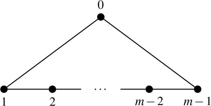
The cyclic quiver.
Starting from this quiver we first take the corresponding doubled quiver. This means that we replace each edge with a pair of edges with opposite orientation to each other. We also equip the quiver with a one-dimensional framing at the vertex 0, and construct the associated Calogero-Moser quiver variety. See Figure 2 for a particular example. The precise procedure of the construction is as follows.
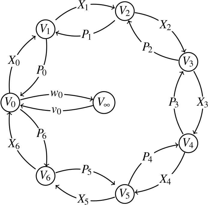
The doubled cyclic quiver for m = 7 with a special framing.
Fix a positive integer n and let V0,V1,...,Vm−1 be vector spaces of dimension n and V∞ be a one-dimensional vector space over the complex field ℂ. Let m stand for the additive group /m of integers modulo m, that is the cyclic group of order m. Let us consider the linear maps
Take the direct sum V = V0 ⊕ V1 ⊕ ···⊕ Vm−1 and define the transformations X,P ∈ End(V) by
Let 1V denote the identity map on V. The commutator [X,P] ∈ End(V) of X and P can be expressed as
Extend v0, w0 introduced in (3.2) to maps v: V∞ → V and w: V → V∞, respectively, by
An m-tuple g =(g0,g1,...,gm−1) ∈ ℂm is called regular if
Let
The group GL(V) ⊂ End(V) of invertible linear transformations acts on
If g is regular, then this action is free. The equivariant Calogero-Moser space
In the rest of the paper we will suppress the dependence of
In [3] Chalykh and Silantyev introduced local coordinates on the open dense subset
By using the group action and the constraint (3.9) they showed that each point of
The maps Mv, wM−1 are expressed as column and row vectors, respectively, with m blocks of size n each. The only non-zero blocks are the first ones, i.e.
It was also proved in [3] that these local coordinates (pj/m,qj) are canonical. That is, the symplectic structure on
The Hamiltonians can be written as
The same procedure can be repeated by introducing local coordinates (λj, ϕj) on the open dense subset
The maps
Finally, the symplectic structure on
The Hamiltonians Hk (3.17), when expressed in terms of (λj, ϕk), take a much simpler form
4. Canonical spectral coordinates in the spinless case
Now we turn to the task of finding explicit formulas for variables conjugate to the eigenvalues λ1,...,λn of Pi, i.e. such functions θ1,...,θn in involution that
It follows from (3.22) that the variables ϕ1/m,..., ϕn/m are such functions. Proposition 4.1 below provides explicit formulas for ϕk in terms of λ. To formulate the statement we need the following functions on
Notice that these functions, besides z, depend only on the class of the quadruple (X,P,v,w) under the GL(V)-action (we have suppressed this dependence). Therefore A,C,D descend to well-defined functions on
Lemma 4.1
The characteristic polynomial A(z)= det(z1V − P) can be written in terms of λ1,...,λn as
Proof.
[Proof #1] Notice that A(z) is invariant under conjugation, i.e. constant along orbits of GL(V). Thus we can use
By iterating this process (m − 2) times we obtain
Applying the determinant formula (4.8) one more time yields
This concludes the proof.
Let us give an alternative and more direct proof.
Proof.
[Proof #2] In this proof we partition the matrix the same way as in (4.7), but apply a different version of the block matrix determinant formula, namely
This requires the calculation of the determinant and inverse of the bottom right block. Fortunately, this block is an upper triangular matrix of size (m − 1)n. Its determinant is
The product βδ−1γ is simply λ2[δ−1]1,m−1. Substituting everything into (4.12) yields
Lemma 4.2
The inverse of z1V − P can be written explicitly in terms of λ1,...,λn as an m × m block matrix with blocks of size n of the form
If one does not wish to use mod m exponents one can write
Proof.
A simple check confirms that the matrix defined by formulas (4.17)–(4.18) is such that
We recall that the adjugate of an invertible linear transformation M can be written as adj(M)= det(M)M−1, hence assuming that z1V − P is invertible we have the following
The next statement gives Theorem 1.1 for the spinless CM space
Proposition 4.1.
For a point
Proof.
Since A(z) and D(z) are both invariant under conjugation by elements of GL(V), using
The function D(z) can be written in terms of λ1,...,λn as
Plugging (4.22) into this formula gives
Substituting z = λk causes all terms with j ≠ k to vanish leaving
Differentiating A(z) with respect to z yields
Putting formulas (4.25) and (4.27) together gives
By using (3.14) a simple calculation reveals that c0 + ⋯ + cm−1 = 0 leaving us with
Next, we will prove the analogue of Sklyanin’s formula [8, 16] in the equivariant case, which provides another set of variables θ1,...,θn conjugate to λ1,...,λn. The result gives Theorem 1.2 for
Proposition 4.2.
For a point
Then θk can be written as
In particular, the variables θ1,...,θn given by (4.31) are conjugate to λ1,...,λn, i.e. we have{θj, θk} = 0 and {λj, θk} = δj,k, j, k = 1,...,n.
Proof.
Let us start with C(z). Using gauge invariance we replace the quadruple (X,P,v,w) by (
Using (4.22) with i = 0 yields
Since
Substituting z = λk into this expression yields
Putting formulas (4.27) and (4.37) together gives
This implies that {λj,θk} = δj,k, j, k = 1,...,n. The partial derivative of fk with respect to λj (j ≠ k) is
5. Calogero-Moser spaces with spin variables and their canonical variables
In this section, we derive the analogues of the results obtained in the previous section to models containing spin variables. Let d be a positive integer. The affine Dynkin quiver
The space itself is denoted as
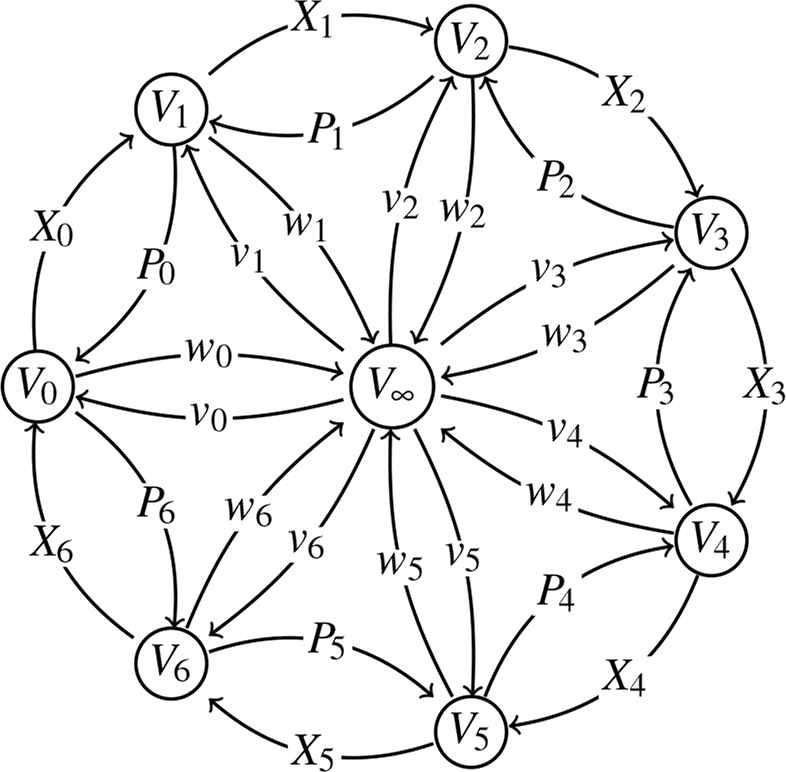
The doubled cyclic quiver for m = 7 with the modified framing.
The objects we are most interested in are the ones corresponding to
The Poisson bracket of two functions f,g on the spin Calogero-Moser space
The expressions of the functions A,C,D on the spin Calogero-Moser space are formally the same as in the spinless case. Namely,
Again, the dependence of them on the class of (X,P,v,w) is suppressed. In the spin case the product vw is understood to be the sum of the tensor (or dyadic) products
The next result gives Theorem 1.1 for the spin case.
Proposition 5.1.
The variables ϕ1,..., ϕn can be expressed using the functions A and D as follows
Proof.
Using expression (4.23) we get
Interchanging the order of summation and the identity
Substituting z = λk into this formula yields
The next statement completes the proof of Theorem 1.2 in the spin case.
Proposition 5.2.
For a point
Then the variables θ1,...,θn given by the generalized Sklyanin’s formula (5.21) are conjugate to λ1,...,λn.
Proof.
A direct calculation shows that
Taking (5.5)–(5.7) into account, the variable θk can be explicitly spelled out as
The explicit expression (5.24) lets us decompose {θj,θk} as follows
Since ϕj and ϕk Poisson commute and ej depends only on λj, but not the other λ’s, each of the first four terms on the right-hand side is zero, that is
Hence we are left with
Indeed, we have
Thus
Rewriting the sum using a new pair of indices h′, i′ given by
Let us consider the first term on the right-hand side. Since ej and fk do not depend on any of the ϕ’s and ej only depends on the j-th column (resp. row) of
A straightforward computation yields
Collecting the common factor
Similarly,
As for the partial derivatives of fk,we have
Putting formulas (5.40)–(5.43) together, {ej, fk} (5.38) is found to be
The Poisson bracket {fj,ek} is obtained from {ej, fk} (5.44) by changing its sign and exchanging j and k. Hence we get
Rewriting this using the new index h ≡ m − h′− 2 (mod m) allows us to collect the factors of the terms with the same λ dependence in {ej, fk} and {fj,ek}. Then we add (5.44) and (5.45) together and find that the terms with ci and
Let us now consider the last term {fj, fk} in {θj, θk} (5.37). Since fj and fk do not depend on any of the ϕ’s we have
We already calculated most of these partial derivatives in (5.42) and (5.43). The only ones remaining are
Fortunately, these expressions are related. For example, we get B if we exchange j and k in A. We denote this by writing that B =(A)j↔k. There are similar relations between the expressions C and F, as well as between the expressions D and E. In short, we have
This observation saves us half the work as we only need to calculate, say A, F, and E. First, we calculate A and find that
Second, we calculate F and get
Third, we calculate E and get
We obtain explicit formulas for B, C, and D from (5.52)–(5.54) and the relations (5.51). Namely,
By a suitable change of indices in D and F we see that in A−D−F almost all terms cancel. The only ones remaining are the terms with ℓ = k in D and the terms with ℓ = j in F. As a consequence, we get
With the same type of computation we obtain
Since the exponents of λj and λk do not depend on i and depend only on the difference of h and h′, but not on the individual indices, introducing a new index h″:= h − h′ and adding (5.58) to (5.59), yields an explicit formula for the Poisson bracket {fj, fk}. Namely, we get
This is the same expression as (5.46) only with opposite sign. Hence these two terms in {θj, θk} cancel and we obtain
Finally, let us observe that due to (5.7) we can take any fixed h ∈ m and β ∈ {1,...,d} and express
Remark 5.1.
Let us list some important special cases of our results. In [3], it was shown that the m = 2, d = 1 case corresponds to the rational Calogero-Moser system of type Bn (and with g1 = 0 of type Dn). Setting m = 1, d > 1 produces the Gibbons-Hermsen system [6], whereas the m = 2, d > 1 case contains the type Bn variant of the Gibbons-Hermsen system.
6. The equivariant geometry of the interpolation curves
Now we briefly describe the geometry of the interpolation curves appearing in Theorems 1.1 and 1.2. These are the affine plane curves
Both of these are rationally parametrized. Hence, they can be completed to rational curves in ℂ2. The expressions (4.26), (4.36), (5.22), (4.24) and (5.18) show that the polynomials A′(z), C(z) and D(z) in all cases are divisible by zm−2. After cancellations we can write
Let Δ be the root system Am−1 and let us choose a primitive m-th root of unity ω. There corresponds to Δ a subgroup GΔ of SL(2, ℂ), a cyclic subgroup of order m, which is generated by the matrix
All irreducible representations of GΔ are one-dimensional, and are given by ρj : σ ↦ ωj, for j ∈ m. The corresponding McKay quiver is the cyclic Dynkin diagram of type
As it was remarked in [3, Section 5.1] the set of eigenvalues (
The following lemma is straightforward from (4.32) and (5.24).
Lemma 6.1
When λi is replaced by ωλi, then θi is replaced by ω−1θi. Therefore, the coordinates λi, θi are also well-defined only up to the action of Sn ⋉ GΔ.
Corollary 6.1.
The pairs of variables (λi,ϕi) and (λi,θi) are well-defined on ℂ2/GΔ.
As a result, the curves C1 and C2 are only well-defined up to the action of GΔ. But they descend to well-defined curves on the quotient space ℂ2/GΔ.
Corollary 6.2.
The curves C1 and C2 descend to well-defined rational curves C1/GΔ and C2/GΔ on ℂ2/GΔ. When considered as a subvariety of ℂ3 = Spec(ℂ [a,b,c]),C1/GΔ and C2/GΔ are given by the intersection of the surface (6.5) and the surface
Conversely, if C ⊂ℂ2/GΔ is a rational curve of degree n which is of the above form, then any distinct n points on it determine a point of
Acknowledgements
We would like to thank Jim Bryan, Maxime Fairon, and Balázs Szendrői for helpful comments and discussions.
This project has received funding from the European Union’s Horizon 2020 research and innovation programme under the Marie Skłodowska-Curie grant agreement No 795471.
References
Cite this article
TY  - JOUR
AU  - Tamás Görbe
AU  - Ádám Gyenge
PY  - 2020
DA  - 2020/01/27
TI  - Canonical spectral coordinates for the Calogero-Moser space associated with the cyclic quiver
JO  - Journal of Nonlinear Mathematical Physics
SP  - 243
EP  - 266
VL  - 27
IS  - 2
SN  - 1776-0852
UR  - https://doi.org/10.1080/14029251.2020.1700634
DO  - 10.1080/14029251.2020.1700634
ID  - Görbe2020
ER  -