The gauge transformation of the modified KP hierarchy

Jipeng Cheng

doi:10.1080/14029251.2018.1440743

<Previous Article In Issue

Download article (PDF)

Next Article In Issue>

Volume 25, Issue 1, February 2018, Pages 66 - 85

The gauge transformation of the modified KP hierarchy

Authors

Jipeng Cheng

Department of Mathematics, China University of Mining and Technology, Xuzhou, Jiangsu 221116, P. R. China, Email:chengjp@cumt.edu.cnandchengjp@mail.ustc.edu.cn

Received 9 June 2017, Accepted 19 August 2017, Available Online 6 January 2021.

DOI: 10.1080/14029251.2018.1440743 How to use a DOI?
Keywords: mKP hierarchy; gauge transformation; tau function
Abstract: In this paper, we firstly investigate the successive applications of three elementary gauge transformation operators T_i with i = 1,2,3 for the mKP hierarchy in Kupershmidt-Kiso version, and find that the gauge transformation operators T_i can not commute with each other. Then two types of gauge transformation operators T_D and T_I constructed from T_i are proved that they can commute with each other. In particular, T_I is introduced for the first time in the literature. And the successive applications of T_D and T_I in the form of T^(n,k), which is the product of n terms of T_D and k terms of T_I, are derived in three cases for different n and k. At last, the corresponding successive applications of T_D and T_I on the eigenfunction Φ, the adjoint eigenfunction Ψ and the tau functions τ₀ and τ₁ are considered.
Copyright: © 2018 The Authors. Published by Atlantis Press and Taylor & Francis
Open Access: This is an open access article distributed under the CC BY-NC 4.0 license (http://creativecommons.org/licenses/by-nc/4.0/).

1. Introduction

The modified Kadomtsev-Petviashvili (mKP) hierarchy is a system of nonlinear differential equations satisfied by the tau functions introduced in the early 1980s in [14, 15]. There are several versions of the Lax representations for mKP hierarchy. All the definitions are trying to transfer the relationship between KdV and mKdV to the KP situation. The first one is known as the nonstandard integrable system, developed by B. A. Kupershmidt and K. Kiso [16–18, 26], which is defined through the modification of the KP hierarchy (“standard case”) ∂tnL=[(Ln)≥0,L] to ∂tnL=[(Ln)≥1,L] (see Section 2 for more details). The second one is defined by the factorization of the Lax operator of the KP hierarchy [6, 19]. The last one has the representation in terms of differential-difference equations [8, 31, 32]. In this paper, we only consider the first one, i.e., Kupershmidt-Kiso version, since it is comparatively easier to discuss the gauge transformation in the first version than other ones. The mKP hierarchy in Kupershmidt-Kiso version is the particular case of the coupled modified KP hierarchy [32], which are proved that there are two tau functions τ₀ and τ₁. These two tau functions bring much difficulty in the study of the mKP hierarchy, compared with the KP case [7] only owning a single tau function.

The gauge transformation [2, 26, 27], also called Darboux transformation, provides a simple way to construct solutions for integrable hierarchies. By now, the gauge transformations of many integrable hierarchies have been studied, for example, the KP and mKP hierarchies [1–3, 9, 26, 27, 29, 30, 34], the BKP and CKP hierarchies [4, 10, 12, 25], the discrete KP and modified discrete KP hierarchies [13, 20, 21, 24, 28], the q−KP and modified q-KP hierarchies [5, 11, 22, 23, 33] and so on. Here in this paper, we will investigate the gauge transformation of the mKP hierarchy in Kupershmidt-Kiso version. There are three elementary gauge transformation operators T_i with i = 1, 2, 3 (see Section 3 for more details) for the mKP hierarchy [26, 29, 30]. Here we find that T_i with i = 1, 2, 3 can not commute with each other and therefore they are inconvenient in the application. Thus two types of gauge transformation operators T_D [26] and T_I constructed from T_i (see Section 4 for more details) are introduced, which are proved that they can commute with each other. And in particular, as far as I know, T_I is introduced for the first time in the literature. These gauge transformation operators can not only construct various solutions, but also provide the understanding of the inner structures of the mKP hierarchy, for example, the explicit forms of the tau functions for the mKP hierarchy in Kupershmidt-Kiso version. The main content of this paper is devoted to the successive applications of T_D and T_I.

In the KP case, there are two elementary gauge transformation operators, denoted by T_d and T_i. As for the successive applications of n terms of T_d and k terms of T_i, it is enough to only discuss two cases of n > k and n = k in the KP hierarchy [9], since the case k > n can be derived from the commutativity of T_d and T_i, and also the fact that the inverse of the conjugation of T_d is T_i and vice versa. However in the mKP case, the inverse of the conjugation of T_D is not equal to T_I and vice versa. Therefore in the mKP case, if we denote the product of n terms of T_D and k terms of T_I as T^(n,k), all three cases for different n and k should be considered in the successive applications of T_D and T_I. Thus the derivation of T^(n,k) in the case of k > n can not be avoided, which is one of the major differences from the corresponding results in the KP hierarchy. In addition, we give the detailed derivations of the assumption of the form of T^(n,k). But just knowing the assumed form of T^(n,k) is not enough in the derivations of explicit form of T^(n,k). Actually, besides the similar conditions of T_D and T_I (see (4.3)) to the KP case, the additional conditions (see (4.4)) are very crucial in this paper, which is another difference from those in the KP case. At last, the corresponding successive applications of T_D and T_I on the eigenfunction Φ, the adjoint eigenfunction Ψ and the tau functions τ₀ and τ₁ are considered. And some examples of τ₀ and τ₁ are given.

This paper is organized in the following way. In Section 2, some basic facts about the mKP hierarchy are introduced. The successive applications and the commutativity of the elementary gauge transformation operators T_i with i = 1, 2, 3 are discussed in Section 3. Then in Section 4, the successive applications of the gauge transformation operators T_D(Φ) and T_I(Ψ) are investigated in three cases for different n and k. Further the application on the (adjoint) eigenfunctions and the tau functions are obtained in Section 5. At last in Section 6, some conclusions and discussions are given.

2. the mKP hierarchy

The mKP hierarchy in Kupershmidt-Kiso version [16–18, 26] is defined as the following Lax equation

∂tnL=[(Ln)≥1,L],n=1,2,3,⋯ (2.1)

with the Lax operator L given by the pseudo-differential operator below

L=∂+u0+u1∂−1+u2∂−2+u3∂−3+⋯, (2.2)

Here ∂ = ∂_x and u_i = u_i(t₁ = x, t₂, ⋯). The algebraic multiplication of ∂ⁱ with the multiplication operator f is given by the usual Leibnitz rule

∂if=∑j≥0(ij)f(j)∂i−j, i∈ℤ, (2.3)

where f(j)=∂jf∂xj . For A=∑iai∂i,A≥k=∑i≥kai∂i and A<k=∑i<kai∂i . The name of the mKP hierarchy comes from the fact that (2.1) contains the mKP equation

4utx=(uxxx−6u2ux)x+3uyy+6uxuy+6uxx∫uydx. (2.4)

In this paper, for any (pseudo-) differential operator A and a function f, the symbol A(f) will indicate the action of A on f, whereas the symbol Af will denote just operator product of A and f, and * stands for the conjugate operation: (AB)^* = B^*A^*, ∂^* = −∂, f^* = f. Note that there is the term u₀ in the Lax operator L (see (2.2)) of the mKP hierarchy, which is different from the case of the KP hierarchy.

Similar to the case of the KP hierarchy, the Lax operator L for the mKP hierarchy can be expressed in terms of the dressing operator Z,

LmKP=Z∂Z−1, (2.5)

where Z is given by

Z=z0+z1∂−1+z2∂−2+⋯(z0−1exists ). (2.6)

Then the Lax equation (2.1) is equivalent to

∂tnZ=−(LmKPn)≤0Z=−(Z∂nZ−1)≤0Z. (2.7)

Define the wave and the adjoint wave functions of the mKP hierarchy in the following way:

w(t,λ)=Z(eξ(t,λ))=w^(t,λ)eξ(t,λ), (2.8)

w*(t,λ)=(Z−1∂−1)*(e−ξ(t,λ))=w^*(t,λ)λ−1e−ξ(t,λ), (2.9)

with

ξ(t,λ)=xλ+t2λ2+t3λ3+⋯, (2.10)

w^(t,λ)=z0+z1λ−1+z2λ−2+⋯, (2.11)

w^*(t,λ)=z0−1+z1*λ−1+z2*λ−2+⋯. (2.12)

Then w(t, λ) and w^*(t, λ) satisfy the bilinear identity [32] below

resλw(t′,λ)w*(t,λ)=1, (2.13)

which is equivalent to the mKP hierarchy. Here resλ∑iaiλi=a−1 .

It is proved in [32] that there exist two tau functions^a τ₁ and τ₀ for the mKP hierarchy in Kupershmidt-Kiso version such that

w(t,λ)=τ0(t−[λ−1])τ1(t)eξ(t,λ), (2.14)

w*(t,λ)=τ1(t+[λ−1])τ0(t)λ−1e−ξ(t,λ). (2.15)

By comparing (2.11) with (2.14), one can find

z0=τ0(t)τ1(t), z1z0=−∂xlnτ0(t). (2.16)

The eigenfunction Φ and the adjoint eigenfunction Ψ of the mKP hierarchy are defined in the identities below,

Φtn=(Ln)≥1(Φ), Ψtn=−(Ln)≥1*(Ψ). (2.17)

3. Elementary Gauge Transformation

In this section, we will investigate the elementary gauge transformation of the mKP hierarchy. For the mKP hierarchy (2.1), suppose T is a pseudo-differential operator, and

L(1)=TLT−1, (3.1)

such that

∂tnL(1)=[(L(1))≥1n,L(1)] (3.2)

still holds for the transformed Lax operator L⁽¹⁾, then T is called a gauge transformation operator of the mKP hierarchy. According to (3.2), one can easily obtain the lemma below.

Lemma 3.1.

If the pseudo-differential operator T satisfies

(TLnT−1)≥1=T(Ln)≥1T−1+TtnT−1, (3.3)

then T is a gauge transformation operator of the mKP hierarchy.

Before the construction of the gauge transformation, the following basic identities on the pseudo-differential operator are needed.

Lemma 3.2.

For any pseudo-differential operator A and arbitrary functions f, f₁, f₂, g, g₁ and g₂, one has the following operator identities:

(f−1Af)≥1=f−1A≥1f−f−1A≥1(f), (3.4)

(fx−1∂A∂−1fx)≥1=fx−1∂A≥1∂−1fx−fx−1(A≥1(f))x, (3.5)

(∂−1gAg−1∂)≥1=∂−1gA≥1g−1∂−∂−1g−1A≥1*(g)∂, (3.6)

(Af∂−1)<0=A≥0(f)∂−1+A<0f∂−1, (3.7)

(∂−1gA)<0=∂−1A≥0*(g)+∂−1gA<0, (3.8)

f1∂−1g1f2∂−1g2=f1∫g1f2dx⋅∂−1g2−f1∂−1∫g1f2dx⋅g2. (3.9)

Proof. (3.4), (3.5), (3.7) and (3.8) can be found in [26, 27]. (3.9) can be obtained by direct computation. Therefore, we only prove (3.6) here. By using (3.8)

(∂−1gAg−1∂)≥1=(∂−1gA≥1g−1)≥0∂=∂−1gA≥1g−1∂−(∂−1gA≥1g−1)<0∂=∂−1gA≥1g−1∂−∂−1g−1A≥1*(g)∂.

After the preparation above, one can find the following proposition [26, 29, 30] about the mKP hierarchy by using Lemma 3.1 and Lemma 3.2.

Proposition 3.1.

There are three elementary gauge transformation operators for the mKP hierarchy, that is,

T1(Φ)=Φ−1, (3.10)

T2(Φ)=Φx−1∂, (3.11)

T3(Ψ)=∂−1Ψ, (3.12)

where Φ ≠ 0 and Ψ are the eigenfunction and the adjoint eigenfunction of the mKP hierarchy (see (2.17)) respectively, and in particular Φ is not a constant in T₂.

Further, one can obtain the following proposition.

Proposition 3.2.

Under the gauge transformation operator T₁(Φ), T₂(Φ) and T₃(Ψ), the objects in the mKP hierarchy are transformed in the way shown in Table I.

LmKP→LmKP(1)	Z⁽¹⁾ =	Φ1(1)=	Ψ1(1)=	τ0(1)=	τ1(1)=
T_{1 =} Φ^{− 1}	Φ^{− 1}Z	Φ^{− 1}Φ₁	ΦΨ₁	τ₀	Φτ₁
T2=Φx−1∂	Φr−1∂Z∂−1	Φx−1Φ1x	Φx∫Ψ1dx	τ₁	Φxτ12/τ0
T3=∂−1Ψ	∂−1ΨZ∂	∫ΨΦ1dx	(Ψ1/Ψ)x	Ψτ02/τ1	τ₀

Table I

Elementary gauge transformations mKP → mKP

where Φ₁ and Ψ₁ are the different eigenfunction and the adjoint eigenfunction of L_mKP from the generating functions Φ and Ψ of the gauge transformation operators.

Proof. Here we only take T₂ as an example and the others can be derived in the similar way. The actions of T₂ on Z, Φ₁ and Ψ₁ can be obtained by direct computation. Therefore we mainly focus on the actions on τ₀ and τ₁. Firstly, from

Z(1)=Φx−1∂Z∂−1=Φx−1∂(z0+z1∂−1+⋯)∂−1=Φx−1z0+Φx−1(z0x+z1)∂−1+⋯, (3.13)

one can get

z0(1)=Φx−1z0, z1(1)=Φx−1(z0x+z1). (3.14)

Then by (2.16), one can find

−∂xlnτ0(1)=z1(1)z0(1)=∂xlnz0+z1z0=∂xlnz0τ0. (3.15)

Therefore according to (2.16) and (3.14),

τ0(1)=τ0z0=τ1, τ1(1)=τ0(1)z0(1)=Φxτ12τ0. (3.16)

Remark: Note that in [29, 30], there is another gauge transformation operator T=∂−1∫Ψdx⋅∂ , which can be viewed as the composition of T₂ and T₃, that is, T₃(Ψ⁽¹⁾)T₂(Φ) = ∂⁻¹ Ψ⁽¹⁾ Φ∂ = ∂−1∫Ψdx⋅∂ , with Ψ⁽¹⁾ = T₂(Φ)(Ψ).

Denote the successive applications of gauge transformation operators T_i with i = 1, 2, 3 as

T1(n)(Φ1,⋯,Φn)≜T1(Φn(n−1))⋯T1(Φ3(2))T1(Φ2(1))T1(Φ1), (3.17)

T2(n)(Φ1,⋯,Φn)≜T2(Φn(n−1))⋯T2(Φ3(2))T2(Φ2(1))T2(Φ1), (3.18)

T3(n)(Ψ1,⋯,Ψn)≜T3(Ψn(n−1))⋯T3(Ψ3(2))T3(Ψ2(1))T3(Ψ1). (3.19)

Here Φ_i and Ψ_i are the eigenfunctions and the adjoint eigenfunctions of the mKP hierarchy which are different from each other, Φk(m)=Ti(m)(Φ1,⋯,Φm)(Φk) and Ψk(m)=Ti(m)(Ψ1,⋯,Ψm)(Ψk) . The results of the successive applications of gauge transformation operators T_i with i = 1, 2, 3 are listed in the proposition below.

Proposition 3.3.

(1)

T1(n)(Φ1,⋯,Φn)=Φn−1, (3.20)

(2)

T2(n)(Φ1,⋯,Φn)=1Wn+1(1,Φ1,⋯,Φn)|Φ1x⋯Φn−1,x∂⋮⋮⋮⋮Φ1(i)⋯Φn−1(i)∂i⋮⋮⋮⋮Φ1(n)⋯Φn−1(n)∂n|, (3.21)

(3)

T3(n)(Ψ1,⋯,Ψn)=(−1)n+1Wn−1(Ψ1,⋯,Ψn−1)|Ψ1Ψ1(1)⋯Ψ1(n−2)∂−1Ψ1⋮⋮⋮⋮⋮ΨnΨn(1)⋯Ψn(n−2)∂−1Ψn|, (3.22)

where W_n ≡ W_n(Φ₁, Φ₂,⋯,Φ_n) is the Wronskian determinant of Φ₁, Φ₂,⋯,Φ_n. And the determinant of T3(n) is expanded by the last column and the functions are on the left-hand side.

Proof. (1)

T1(n)=T1(Φn(n−1))⋯T1(Φ3(2))T1(Φ2(1))T1(Φ1)=(Φ1Φ2(1)⋯Φn−2(n−3)Φn−1(n−2)Φn(n−1))−1=(Φ1Φ2(1)⋯Φn−2(n−3)Φn(n−2))−1=(Φ1Φ2(1)⋯Φn(n−3))−1=⋯=Φn−1, (3.23)

where we have used the following fact Φk(k−1)Φj(k)=Φj(k−1) , with Φj(k)=T1(Φk(k−1))(Φj(k−1)) .

(2) Assume T2(n)=∑i=1nai∂i . Since T2(n)(Φi)=0,i=1,2,⋯,n−1 and T2(n)(Φn)=1 , one can obtain the following linear equation group,

{∑i=1naiΦk(i)=0, k=1,2,⋯n−1,∑i=1naiΦn(i)=1. (3.24)

Thus

ai=(−1)i+n1Wn+1(1,Φ1,⋯,Φn)|Φ1x⋯Φn−1,x⋮⋮⋮Φ1(i−1)⋯Φn−1(i−1)Φ1(i+1)⋯Φn−1(i+1)⋮⋮⋮Φ1(n)⋯Φn−1(n)|. (3.25)

The substitution of (3.25) for T2(n)=∑i=1nai∂i leads to (3.21).

(3) Firstly, we can prove that T3(n) has the form of T3(n)=∑i=1nbi∂−1Ψi with bn=(−1)n+1 by induction. In fact, we can assume T3(n−1)(Ψ2(1),⋯,Ψn(1))=∑i=2nbi∂−1Ψi(1) with b_n = (−1)ⁿ. Then according to (3.9) and Proposition 3.2, one can find

T3(n)=T3(n−1)(Ψ2(1),⋯,Ψn(1))T3(Ψ1)=∑i=2nbi∂−1Ψi(1)∂−1Ψ1 =∑i=2n(bi∫Ψi(1)dx⋅∂−1Ψ1−bi∂−1∫Ψi(1)dx⋅Ψ1) =∑i=2n(bi∫Ψi(1)dx⋅∂−1Ψ1−bi∂−1Ψi) (3.26)

still holds with the term (−1)ⁿ ^{+ 1}∂⁻¹Ψ_n.

Then by comparing the fact T3(n)=α−n∂−n+ (lower order terms) with the form of T3(n) given above, one can obtain the following linear equation group,

{∑i=1nbiΨi(k)=0, k=0,1,2,⋯n−2,bn=(−1)n+1. (3.27)

Therefore

bi=(−1)i+1Wn−1(Ψ1,⋯,Ψn−1)|Ψ1⋯Ψi−1Ψi+1⋯ΨnΨ1x⋯Ψi−1,xΨi+1,x⋯Ψn,x⋮⋮⋮⋮⋮⋮Ψ1(n−2)⋯Ψi−1(n−2)Ψi+1(n−2)⋯Ψn(n−2)|, (3.28)

which leads to (3.22).

Assume L be the Lax operator of the mKP hierarchy, Φ₁ and Φ₂ be two nonzero independent eigenfunctions, and Ψ₁ and Ψ₂ be two independent adjoint eigenfunctions. we consider the following diagram

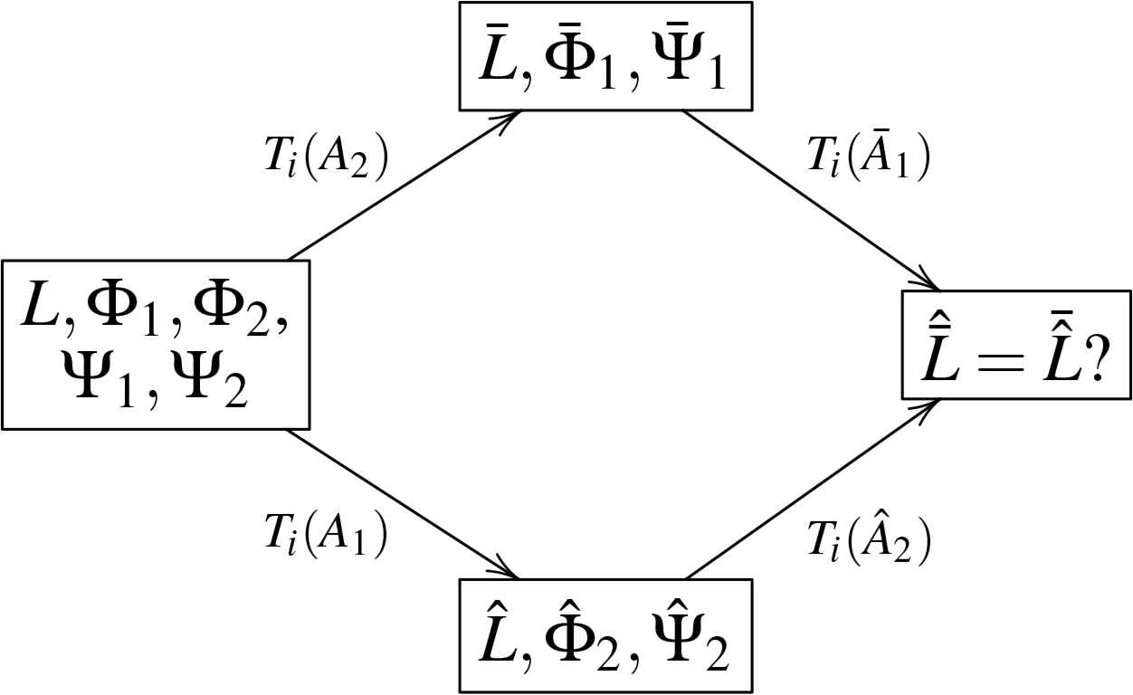
where i = 1, 2, 3 and

Ai={Φ,i=1,2Ψ,i=3,L^=Ti(A1)LTi(A1)−1, Φ^2=Ti(A1)(Φ2), Ψ^2=(Ti*(A1))−1(Ψ2),L¯=Ti(A2)LTi(A2)−1, Φ¯1=Ti(A2)(Φ1), Ψ¯1=(Ti*(A2))−1(Ψ1),L¯^=Ti(A¯1)L¯Ti(A¯1)−1, L^¯=Ti(A^2)L^Ti(A^2)−1. (3.29)

The question is whether this diagram will commute, i.e.

Ti(2)(Φ1,Φ2)=Ti(2)(Φ2,Φ1), i=1,2,T3(2)(Ψ1,Ψ2)=T3(2)(Ψ2,Ψ1). (3.30)

In fact, according to Proposition 3.3,

T1(2)(Φ1,Φ2)−T1(2)(Φ2,Φ1)=Φ2−1−Φ1−1≠0, (3.31)

T2(2)(Φ1,Φ2)−T2(2)(Φ2,Φ1)=1W3(1,Φ1,Φ2)|Φ1x+Φ2x∂Φ1xx+Φ2xx∂2|≠0, (3.32)

T3(2)(Ψ1,Ψ2)−T3(2)(Ψ2,Ψ1)=(Ψ2/Ψ1+1)∂−1Ψ1−(Ψ1/Ψ2+1)∂−1Ψ2≠0. (3.33)

Therefore, the Bianchi diagrams for T_i, i = 1, 2, 3 does not commute. Further, according to Proposition 3.2, one can also find that

T1(Φ2(1))T2(Φ1)≠T2(Φ1(1))T1(Φ2), (3.34)

T1(Φ(1))T3(Ψ)≠T3(Ψ(1))T1(Φ), (3.35)

T2(Φ(1))T3(Ψ)≠T3(Ψ(1))T2(Φ). (3.36)

So T_i with i = 1, 2, 3 can not commute with each other, that is,

TiTj≠TjTi, i,j=1,2,3. (3.37)

This fact tells us that the gauge transformation operators T_i with i = 1, 2, 3 are not convenient when solving the mKP hierarchy. Thus we must seek the other kinds of gauge transformation operators which can commute with each other in the mKP hierarchy, that is, T_D(Φ) and T_I(Ψ).

4. Gauge Transformation operators T_D(Φ) and T_I(Ψ)

Since 1 is the eigenfunction of the mKP hierarchy (see (2.17)), one can define

TD(Φ)≜T2(1(1))T1(Φ)=(Φ−1)x−1∂Φ−1, (4.1)

TI(Ψ)≜T1(1(1))T3(Ψ)=(∫Ψdx)−1∂−1Ψ. (4.2)

Here T_D is introduced in [26], while as far as I know T_I is presented for the first time in the literature. Then by the direct computation similar to Proposition 3.2, one can obtain the following proposition.

Proposition 4.1.

Under the gauge transformation operator T_D(Φ) and T_I(Ψ), the objects in the mKP hierarchy are transformed in the way shown in Table II.

LmKP→LmKP(1)	Z⁽¹⁾ =	Φ1(1)=	Ψ1(1)=	τ0(1)=	τ1(1)=
T_D(Φ)	T_D(Φ)Z∂^{− 1}	(Φ1/Φ)x/(Φ−1)x	(Φ−1)x⋅∫ΦΨ1dx	Φτ₁	−Φxτ12/τ0
T₁(Ψ)	T₁(Ψ)Z∂	∫ΨΦ1dx/∫Ψdx	(Ψ1/Ψ)x⋅∫Ψdx	Ψτ02/τ1	τ0⋅∫Ψdx

Table II

gauge transformations T_D(Φ) and T_I(Ψ)

According to Table II, one finds that

TD(Φ)(Φ)=0, (TI(Ψ)−1)*(Ψ)=0, (4.3)

TD(Φ)(1)=1, TI(Ψ)(1)=1. (4.4)

It can be proved that T_D(Φ) and T_I(Ψ) are commute with each other, i.e.,

TD(Φ2(1))TD(Φ1(0))=TD(Φ1(1))TD(Φ2(0)), (4.5)

TD(Φ(1))TI(Ψ(0))=TI(Ψ(1))TD(Φ(0)), (4.6)

TI(Ψ2(1))TI(Ψ1(0))=TI(Ψ1(1))TI(Ψ2(0)). (4.7)

Therefore, T_D(Φ) and T_I(Ψ) are more applicable in the case of the mKP hierarchy.

Consider the following chain of the gauge transformation operators T_D(Φ) and T_I(Ψ)

L→TD(Φ1)L(1)→TD(Φ2(1))L(2)→⋯→L(n−1)→TD(Φn(n−1))L(n)→TI(Ψ1(n))L(n+1)→TI(Ψ1(n+1))⋯→L(n+k−1)→TI(Ψk(n+k−1))L(n+k).

Denote

T(n,k)=TI(Ψk(n+k−1))⋯TI(Ψ1(n))TD(Φn(n−1))⋯TD(Φ2(1))TD(Φ1). (4.8)

Next, we will compute the explicit form of T^(n,k) in terms of Φ_i and Ψ_i. Before this, the lemma below is needed.

Lemma 4.1.

T^{(0, k)} and T^(n,0) have the following form

T(0,k)=∑i=1kαi∂−1Ψi, (4.9)

(T(n,0))−1=∑i=1nΦi∂−1βi. (4.10)

Proof. This lemma can be proved by induction. Here we only prove the first identity, since the second one is almost the same. Assume this lemma holds for k − 1, then according to (3.9) and Table II

T(0,k)=∑i=2kαi∂−1Ψi(1)⋅(∫Ψ1dx)−1⋅∂−1Ψ1 =∑i=2kαi⋅∫(Ψi(1)(∫Ψ1dx)−1)dx⋅∂−1Ψ1 −∑i=2kαi∂−1⋅∫(Ψi(1)(∫Ψ1dx)−1)dx⋅Ψ1 =∑i=2k(αiΨi/Ψ1∂−1Ψ1−αi∂−1Ψi), (4.11)

by noting that

∫(Ψi(1)(∫Ψ1dx)−1)dx⋅Ψ1=Ψi. (4.12)

The generalized Wronskian determinant [9] is needed in the next propositions, which is defined in the following form

IWk,n≡IWk,n(Ψk,Ψk−1,⋯,Ψ1;Φ1,⋯,Φn)=|∫Φ1Ψkdx∫Φ2Ψkdx⋯∫ΦnΨkdx∫Φ1Ψk−1dx∫Φ2Ψk−1dx⋯∫ΦnΨk−1dx⋮⋮⋮⋮∫Φ1Ψ1dx∫Φ2Ψ1dx⋯∫ΦnΨ1dxΦ1Φ2⋯ΦnΦ1xΦ2x⋯Φnx⋮⋮⋮⋮Φ1(n−k−1)Φ2(n−k−1)⋯Φn(n−k−1)|.

In particular,

IW0,n=Wn(Φ1,Φ2,⋯,Φn), (4.13)

which is Wronskian determinant of Φ₁, Φ₂,⋯, Φ_n.

Proposition 4.2.

When n > k, T^(n,k) and (T^(n,k⁾) ^{− 1} have the following forms

T(n,k)=1IWk,n+1(Ψk,Ψk−1,⋯,Ψ1;Φ1,⋯,Φn,1)|∫Φ1Ψkdx∫Φ2Ψkdx⋯∫ΦnΨkdx∂−1Ψk∫Φ1Ψk−1dx∫Φ2Ψk−1dx⋯∫ΦnΨk−1dx∂−1Ψk−1⋮⋮⋮⋮⋮∫Φ1Ψ1dx∫Φ2Ψ1dx⋯∫ΦnΨ1dx∂−1Ψ1Φ1Φ2⋯Φn1Φ1xΦ2x⋯Φnx∂⋮⋮⋮⋮⋮Φ1(n−k)Φ2(n−k)⋯Φn(n−k)∂n−k| (4.14)

and

(T(n,k))−1=(−1)n−1IWk,n+1(Ψk,Ψk−1,⋯,Ψ1;Φ1,⋯,Φn,1)IWk,n(Ψk,Ψk−1,⋯,Ψ1;Φ1,⋯,Φn)2|Φ1∂−1∫ΨkΦ1dx⋯∫Ψ1Φ1dxΦ1⋯Φ1(n−k−2)Φ2∂−1∫ΨkΦ2dx⋯∫Ψ1Φ2dxΦ2⋯Φ2(n−k−2)⋮⋮⋮⋮⋮⋮⋮Φn∂−1∫ΨkΦndx⋯∫Ψ1ΦndxΦn⋯Φn(n−k−2)|. (4.15)

Here the determinant of T^(n,k) is expanded by the last column and the functions are on the left-hand side. And when computing (T^(n,k))⁻¹, the determinant of (T^(n,k)) ^{− 1} is expanded by the first column and the functions are on the right-hand side, and also the coefficient function before the determinant should be placed after the operators Φ_i∂ ^{− 1}.

Proof. When n > k, according to (4.8) and the commutativity of T_D and T_I given in (4.5)–(4.7), one can rewrite T^(n,k) as

T(n,k)=AT(0,k)=B−1T(n,0), (4.16)

where

A=TD(Φn(n+k−1))⋯TD(Φ2(k+1))TD(Φ1(k)), (4.17)

B=(TI(Ψk(n+k−1))TI(Ψk−1(n+k−2))⋯TI(Ψ1(n)))−1. (4.18)

Then by using Lemma 3.2 and Lemma 4.1, and also the fact (T(n,k))−1=((T(n,k))−1)− ,

(T(n,k))−=(AT(0,k))−=(A∑i=1kαi∂−1Ψi)−=∑i=1kA(αi)∂−1Ψi, (4.19)

(T(n,k))−1=((T(n,0))−1B)−=(∑i=1nΦi∂−1βiB)−=∑i=1nΦi∂−1B*(βi). (4.20)

Thus T^(n,k) and (T^(n,k)) ^{− 1} have the following forms

T(n,k)=∑i=0n−kai∂i+∑i=−k−1ai∂−1Ψ−i, (4.21)

(T(n,k))−1=∑j=1nΦj∂−1bj, (4.22)

where a_i and b_j are the functions that will be determined below.

Then from Table II, one can find

T(n,k)(Φi)=0,T(n,k)(1)=1, i=1,2,⋯,n, (4.23)

that is

{∑i=0n−kaiΦj(i)+∑i=−k−1ai∫Ψ−iΦjdx=0, j=1,2,⋯,n,a0+∑i=−k−1ai∫Ψ−idx=1, (4.24)

where (4.21) is used. By solving this equation, (4.14) can be proved.

On the other hand, (4.21), (4.22) and Table II can lead to

((T(n,k))−1)*=∑l=0+∞(−1)l+1∑j=1nbjΦj(l)∂−1−l, (4.25)

((T(n,k))−1)*=(−1)n−kan−k−1∂−n+k+(lower order terms), (4.26)

((T(n,k))−1)*(Ψj)=0, (4.27)

Thus

{∑i=1nbi∫ΦiΨjdx=0, j=k,k−1,⋯,1,∑i=1nbiΦi(j)=0, j=0,1,2,⋯,n−k−2,∑i=1nbiΦi(n−k−1)=an−k−1=IWk,n+1(Ψk,Ψk−1,⋯,Ψ1;Φ1,⋯,Φn,1)IWk,n(Ψk,Ψk−1,⋯,Ψ1;Φ1,⋯,Φn), (4.28)

which gives rise to (4.15).

By the same manner as the case n > k, one can show that T^(n,n) and (T^(n,n))⁻¹ have the similar forms

T(n,n)=a0+∑i=−n−1ai∂−1Ψ−i, (4.29)

(T(n,n))−1=a0−1+∑j=1nΦj∂−1bj, (4.30)

and thus have the following proposition.

Proposition 4.3.

When n = k, T^(n,k) and (T^(n,k)) ^{− 1} have the following forms

T(n,n)=1IWn,n+1(Ψn,Ψn−1,⋯,Ψ1;Φ1,⋯,Φn,1)|∫Φ1Ψndx∫Φ2Ψndx⋯∫ΦnΨndx∂−1Ψn∫Φ1Ψn−1dx∫Φ2Ψn−1dx⋯∫ΦnΨn−1dx∂−1Ψn−1⋮⋮⋮⋮⋮∫Φ1Ψ1dx∫Φ2Ψ1dx⋯∫ΦnΨ1dx∂−1Ψ1Φ1Φ2⋯Φn1|, (4.31)

and

(T(n,n))−1=−IWn,n+1(Ψn,Ψn−1,⋯,Ψ1;Φ1,⋯,Φn,1)IWn,n(Ψn,Ψn−1,⋯,Ψ1;Φ1,⋯,Φn)2|−1ΨnΨn−1⋯Ψ1Φ1∂−1∫ΨnΦ1dx∫Ψn−1Φ1dx⋯∫Ψ1Φ1dxΦ2∂−1∫ΨnΦ2dx∫Ψn−1Φ2dx⋯∫Ψ1Φ2dx⋮⋮⋮⋮⋮Φn∂−1ΨnΦndx∫Ψn−1Φndx⋯∫Ψ1Φndx|. (4.32)

Here the determinant of T^(n,k) is expanded by the last column and the functions are on the left-hand side. And when computing (T^(n,k))⁻¹, the determinant of (T^(n,k)) ^{− 1} is expanded by the first column and the functions are on the right-hand side, and also the coefficient function before the determinant should be placed after the operators Φ_i∂^{− 1}.

As for the case n < k, one has the proposition below.

Proposition 4.4.

When n < k, T^(n,k) and (T^(n,k)) ^{− 1} have the following forms

T(n,k)=(−1)k−1IWn+1,k(1,Φn,Φn−1,⋯,Φ1;Ψ1,⋯,Ψk) |∫ΦnΨ1dx⋯∫Φ1Ψ1dxΨ1⋯Ψ1(k−n−2)∂−1Ψ1∫ΦnΨ2dx⋯∫Φ1Ψ2dxΨ2⋯Ψ2(k−n−2)∂−1Ψ2⋮⋮⋮⋮⋮⋮⋮∫ΦnΨkdx⋯∫Φ1ΨkdxΨk⋯Ψk(k−n−2)∂−1Ψk|, (4.33)

and

(T(n,k))−1=IWn+1,k(1,Φn,Φn−1,⋯,Φ1;Ψ1,⋯,Ψk)IWn,k(Φn,Φn−1,⋯,Φ1;Ψ1,⋯,Ψk)2 |−Φn∂−1∫ΦnΨ1dx⋯∫ΦnΨkdx⋮⋮⋮⋮−Φ1∂−1∫Φ1Ψ1dx⋯∫Φ1Ψkdx1Ψ1⋯Ψk−∂Ψ1x⋯Ψkx⋮⋮⋮⋮(−∂)k−nΨ1(k−n)⋯Ψk(k−n)|. (4.34)

Here the determinant of T^(n,k) is expanded by the last column and the functions are on the left-hand side. And when computing (T^(n,k)) ^{− 1}, the determinant of (T^(n,k⁾) ^{− 1} is expanded by the first column and the functions are on the right-hand side, and also the coefficient function before the determinant should be placed after the operators Φ_i∂⁻ ¹ and ∂ⁱ.

Proof. Firstly when n < k, T^(n,k) and (T^(n,k))⁻¹ have the following forms

T(n,k)=∑i=1kai∂−1Ψi, (4.35)

(T(n,k))−1=∑j=0k−n∂jbj+∑j=1nΦj∂−1b−j, (4.36)

which can be obtained in the same way as the case n>k. Then by using Table II

T(n,k)(Φi)=0, T(n,k)(1)=1, (4.37)

T(n,k)=αn−k∂n−k+(lower order terms)=∑j=0∞(−1)j∑i=1kaiΨi(j)∂−1−j. (4.38)

Therefore

{∑i=1kai∫Ψidx=1,∑i=1kai∫ΨiΦjdx=0, j=n,n−1,⋯,1,∑i=1kaiΨi(j)=0, j=0,1,⋯,k−n−2. (4.39)

By solving this equation, (4.33) can be derived. And also by using

αn−k=∑i=1k(−1)−1+k−naiΨi(−1+k−n), (4.40)

one can obtain

αn−k=(−1)nIWnk(Φn,Φn−1,⋯,Φ1;Ψ1,⋯,Ψk)IWn+1,k(1,Φn,Φn−1,⋯,Φ1;Ψ1,⋯,Ψk). (4.41)

On the other hand, from (4.38), (4.41) and Table II,

((T(n,k))−1)*(Ψi)=0, i=1,2,⋯,k, (4.42)

bk−n=αn−k−1=(−1)nIWn+1,k(1,Φn,Φn−1,⋯,Φ1;Ψ1,⋯,Ψk)IWn,k(Φn,Φn−1,⋯,Φ1;Ψ1,⋯,Ψk). (4.43)

Then

{∑i=0k−n(−1)ibiΨj(i)−∑i=1nb−i∫ΦiΨjdx=0, j=1,2,⋯,k,bk−n=(−1)nIWn+1,k(1,Φn,Φn−1,⋯,Φ1;Ψ1,⋯,Ψk)IWn,k(Φn,Φn−1,⋯,Φ1;Ψ1,⋯,Ψk), (4.44)

which leads to (4.34).

5. Applications of T^(n,k)

In the last section, the explicit forms of T^(n,k) have been obtained. In this section, we will investigate the applications of the above explicit formulas.

Firstly, let’s consider the applications of T^(n,k) on the eigenfunction and adjoint eigenfunction of the mKP hierarchy. We summarize the corresponding results in the next proposition.

Proposition 5.1.

Under the successive gauge transformation T^(n,k), the eigenfunction Φ (which is not proportional to Φ₁, ⋯, Φ_n in T^(n,k)) and the adjoint eigenfunction Ψ (which is not proportional to Ψ₁, ⋯, Ψ_k in T^(n,k)) of the mKP hierarchy will become into

•
when n > k,
Φ(n+k)=IWk,n+1(Ψk,Ψk−1,⋯,Ψ1;Φ1,⋯,Φn,Φ)IWk,n+1(Ψk,Ψk−1,⋯,Ψ1;Φ1,⋯,Φn,1) (5.1)

Ψ(n+k)=(−1)n+1IWk,n+1(Ψk,Ψk−1,⋯,Ψ1;Φ1,⋯,Φn,1)IWk,n(Ψk,Ψk−1,⋯,Ψ1;Φ1,⋯,Φn)2 (5.2)

×IWk+1,n(Ψ,Ψk,⋯,Ψ1;Φ1,⋯,Φn) (5.3)
•
when n = k
Φ(n+n)=IWn,n+1(Ψn,Ψn−1,⋯,Ψ1;Φ1,⋯,Φn,Φ)IWn,n+1(Ψn,Ψn−1,⋯,Ψ1;Φ1,⋯,Φn,1) (5.4)

Ψ(n+n)=(−1)n+1IWn,n+1(Ψn,Ψn−1,⋯,Ψ1;Φ1,⋯,Φn,1)IWn,n(Ψn,Ψn−1,⋯,Ψ1;Φ1,⋯,Φn)2×IWn,n+1(Φ1,⋯,Φn;Ψ,Ψn,⋯,Ψ1). (5.5)
•
when n < k
Φ(n+k)=IWn+1,k(Φ,Φn,⋯,Φ1;Ψ1,⋯,Ψk)IWn+1,k(1,Φn,⋯,Φ1;Ψ1,⋯,Ψk), (5.6)

Ψ(n,k)=−IWn+1,k(1,Φn,Φn−1,⋯,Φ1;Ψ1,⋯,Ψk)IWn,k(Φn,Φn−1,⋯,Φ1;Ψ1,⋯,Ψk)2×IWn,k+1(Φn,⋯,Φ1;Ψ,Ψ1,⋯,Ψk). (5.7)

Proof. These results can be obtained by substituting (4.14), (4.15), (4.31), (4.32), (4.33) and (4.34) into the following expressions
Φ(n+k)=T(n,k)(Φ), Ψ(n+k)=−((T(n,k))−1)*(Ψ). (5.8)

Proposition 5.2.

Under the successive gauge transformation T^(n,k), the tau functions τ₀ and τ₁ of the mKP hierarchy will be changed into

•
when n ≥ k
τ0(n+k)=IWk,n(Ψk,Ψk−1,⋯,Ψ1;Φ1,⋯,Φn)τ1n−kτ0n−k−1, (5.9)

τ1(n+k)=IWk,n+1(Ψk,Ψk−1,⋯,Ψ1;Φ1,⋯,Φn,1)τ1n−k+1τ0n−k; (5.10)
•
when n < k
τ0(n+k)=IWn,k(Φn,Φn−1,⋯,Φ1;Ψ1,⋯,Ψk)τ1n−kτ0n−k−1, (5.11)

τ1(n+k)=(−1)nIWn+1,k(1,Φn,Φn−1,⋯,Φ1;Ψ1,⋯,Ψk)τ1n−k+1τ0n−k. (5.12)

Proof. Here we only give the proof for the case of n ≥ k, since the proof in the other case is almost the same. For this, assume

T(n,k)=αn−k∂n−k+αn−k−1∂n−k−1+⋯. (5.13)

Then through (4.14) and (4.31), one can find

αn−k=IWk,n(Ψk,Ψk−1,⋯,Ψ1;Φ1,⋯,Φn)IWk,n+1(Ψk,Ψk−1,⋯,Ψ1;Φ1,⋯,Φn,1),

αn−k−1=−∂x(IWk,n(Ψk,Ψk−1,⋯,Ψ1;Φ1,⋯,Φn))IWk,n+1(Ψk,Ψk−1,⋯,Ψ1;Φ1,⋯,Φn,1). (5.14)

Further from the transformation

Z(n+k)=T(n,k)Z(0)∂k−n, (5.15)

one can obtain

z0(n+k)=αn−kz0,z1(n+k)=αn−kz1+(n−k)αn−kz0x+αn−k−1z0. (5.16)

Then according to (5.14) and the relation between τ₀ and τ₁ given in (2.16), one can find

−∂xln(τ0(n+k))=z1(n+k)z0(n+k)=z1z0+(n−k)∂xln(z0)+αn−k−1αn−k=−∂xln(τ0)+(n−k)∂xln(z0)−∂xln(IWk,n(Ψk,Ψk−1,⋯,Ψ1;Φ1,⋯,Φn)),

Therefore by (2.16), (5.14) and (5.16),

τ0(n+k)=IWk,n(Ψk,⋯,Ψ1;Φ1,⋯,Φn)τ0z0n−k=IWk,n(Ψk,⋯,Ψ1;Φ1,⋯,Φn)τ1n−kτ0n−k−1,τ1(n+k)=τ0(n+k)z0(n+k)=IWk,n+1(Ψk,Ψk−1,⋯,Ψ1;Φ1,⋯,Φn,1)τ1n−k+1τ0n−k.

In order to obtain the explicit examples of τ₀ and τ₁, we start from the zero solution, i.e., L⁽⁰⁾ = ∂, which satisfies (2.1). One can easily find that in this case, the mKP hierarchy in Kupershmidt-Kiso version coincides with the usual KP hierarchy. Denote

Φi(0)=exp(ξ(t,αi))+aiexp(ξ(t,βi)), i=1,2,⋯,n, (5.17)

Ψj(0)=exp(−ξ(t,γj))+bjexp(−ξ(t,δj)), j=1,2,⋯,k, (5.18)

where α_i, β_i, γ_j and δ_j are distinct complex numbers for different i or j, and a_i and b_j are constants. Then one can easily check that Φi(0) and Ψj(0) satisfy (2.17), and thus Φi(0) and Ψj(0) are the corresponding (adjoint) eigenfunctions of the mKP hierarchy in Kupershmidt-Kiso version or the usual KP hierarchy with respect to L⁽⁰⁾. And in particular, 1 is also the eigenfunction of the KP hierarchy corresponding to L⁽⁰⁾. As for the tau functions in this case, one can easily find that

τ0(0)=1, τ1(0)=1. (5.19)

Then according to Proposition 5.2 and [9], one has the following results

Proposition 5.3.

Starting from the zero solution of the mKP hierarchy, i.e., L⁽⁰⁾ = ∂, the tau pair (τ₀^{(n +k)}, τ₁^{(n +k)}) of the mKP hierarchy is showed as follows.

•
when n ≥ k,
τ0(n+k)=IWk,n(Ψk(0),Ψk−1(0),⋯,Ψ1(0);Φ1(0),⋯,Φn(0)), (5.20)

τ1(n+k)=IWk,n+1(Ψk(0),Ψk−1(0),⋯,Ψ1(0);Φ1(0),⋯,Φn(0),1); (5.21)
•
when n < k
τ0(n+k)=IWnk(Φn(0),Φn−1(0),⋯,Φ1(0);Ψ1(0),⋯,Ψk), (5.22)

τ1(n+k)=(−1)nIWn+1,k(1,Φn,Φn−1,⋯,Φ1;Ψ1,⋯,Ψk). (5.23)

Thus τ0(n+k) and τ1(n+k) can be viewed as the tau functions of the KP hierarchy.

Corollary 5.1.

Starting from L⁽⁰⁾ = ∂, the tau pair (τ0(n),τ1(n)) of the mKP hierarchy is listed below,

τ0(n)=Wn(Φ1(0),⋯,Φn(0)), (5.24)

τ1(n)=Wn+1(Φ1(0),⋯,Φn(0),1); (5.25)

which are also the tau functions of the KP hierarchy.

Remark: the above results can help us to understand the tau pair (τ₀, τ₁) of the mKP hierarchy in Kupershmidt-Kiso version.

6. Conclusions and Discussions

The elementary gauge transformation operators T_i with i = 1, 2, 3 (see Proposition 3.1) are discussed in Section 2. The actions of T_i on the dressing operator, the (adjoint) eigenfunctions and the tau functions are presented in Proposition 3.2. Then the successive applications of gauge transformation operators T_i are shown in Proposition 3.3. At the end of Section 2, T_i are proved that they can not commute with each other (see (3.37)), which reflects that T_i are not easy to carry out for the mKP hierarchy.

Therefore T_D and T_I (see (4.1) and (4.2)) are introduced in Section 3. And in particular, as far as I know, T_I is introduced for the first time in the literature. After that, how the objects of the mKP hierarchy are transformed under T_D and T_I are listed in Proposition 4.1. And further based upon the results in Proposition 4.1, T_D and T_I are shown that they can commute with each other (see (4.5)–(4.7)) and hence they are more applicable in the mKP hierarchy than T_i with i = 1, 2, 3. Then the main part of Section 3 is devoted to the successive applications of T_D and T_I. And the products of n terms of T_D and k-terms of T_I, denoted as T^(n,k), are given in Proposition 4.2 for n > k, Proposition 4.3 for n = k and Proposition 4.4 for n < k. At last, the actions of T^(n,k) on the eigenfunction Φ, the adjoint eigenfunction Ψ and the tau functions τ₀ and τ₁ are presented in Proposition 5.1 and 5.2 Also the explicit forms of tau functions τ₀ and τ₁ are given in Proposition 5.3 and Corollary 5.1.

Compared with the KP hierarchy, there are several differences in the mKP hierarchy, which brings much difficulty to the study of the mKP hierarchy. 1) There is the second high order term in the Lax operator of the mKP hierarchy (see u₀ in (2.2)), which leads to the extra condition (see (4.4)) to determine T^(n,k). 2) The inverse of the conjugation of T_D is not T_I and vice versa. Therefore, the case k > n must be discussed in the derivation of T^(n,k). In fact, it is more difficult in the case k>n than the cases n>k and n = k, because it is very hard to determine the form of T^(n,k) in the case k > n. 3) There are two tau functions τ₀ and τ₁ in the mKP hierarchy. Usually, it is more inconvenient to study the integrable systems with two tau functions than those with only one single tau function. Hence, additional methods must be developed in the discussion of the tau functions under the successive applications of T_D and T_I for the mKP hierarchy.

At last, the results in this paper are hoped to be generalized to the constrained mKP hierarchy. Also these results may be helpful to discuss the inner integrability of the mKP hierarchy such as the additional symmetries and the squared eigenfunction symmetries.

Acknowledgments

This work is supported by the Fundamental Research Funds for the Central Universities (Grant No. 2015 QNA 43).

Footnotes

a

Please note that the mKP hierarchy that we consider is the Kupershmidt-Kiso version, which is different from from those in L. A. Dickey’s work about mKP hierarchy [8]. The existence of τ₁ and τ₀ makes the mKP hierarchy in Kupershmidt-Kiso version become a relatively separate system, just like the KP hierarchy.

References

[1]H Aratyn, E Nissimov, and S Pacheva, Darboux-Backlund solutions of SL(p,q) KP-KdV hierarchies, constrained generalized Toda lattices, and two-matrix string model, Phys. Lett. A, Vol. 201, 1995, pp. 293-305.

[2]LL Chau, JC Shaw, and HC Yen, Solving the KP hierarchy by gauge transformations, Commun. Math. Phys., Vol. 149, 1992, pp. 263-278.

[3]LL Chau, JC Shaw, and MH Tu, Solving the constrained KP hierarchy by gauge transformations, J. Math. Phys., Vol. 38, 1997, pp. 4128-4137.

[4]JP Cheng and JS He, The applications of the gauge transformation for the BKP hierarchy, J. Math. Anal. Appl., Vol. 410, 2014, pp. 989-1001.

[5]JP Cheng, JZ Wang, and XY Zhang, The gauge transformation of the q-deformed modified KP hierarchy, J. Nonlin. Math. Phys., Vol. 21, 2014, pp. 533-542.

[6]Y Cheng, Modifying the KP, the nth constrained KP hierarchies and their Hamiltonian structures, Commun. Math. Phys., Vol. 171, 1995, pp. 661-682.

[7]E Date, M Jimbo, M Kashiwara, and T Miwa, Transformation groups for soliton equations, M Jimbo and T Miwa (editors), Nonlinear integrable systems - classical theory and quantum theory, World Scientific, Singapore, 1983, pp. 39-119.

[8]LA Dickey, Modified KP and discrete KP, Lett. Math. Phys., Vol. 48, 1999, pp. 277-289.

[9]JS He, YS Li, and Y Cheng, The determinant representation of the gauge transformation operators, Chin. Ann. Math. B, Vol. 23, 2002, pp. 475-486.

[10]JS He, Y Cheng, and RA Roemer, Solving bi-directional soliton equations in the KP hierarchy by gauge transformation, J. High Energy Phys., Vol. 03, 2006, pp. 103.

[11]JS He, YH Li, and Y Cheng, q-deformed KP hierarchy and q-Deformed constrained KP hierarchy, SIGMA, Vol. 2, 2006, pp. 060.

[12]JS He, ZW Wu, and Y Cheng, Gauge transformations for the constrained CKP and BKP hierarchies, J. Math. Phys., Vol. 48, 2007, pp. 113519.

[13]R Huang, T Song, and CZ Li, Gauge transformations of constrained discrete modified KP systems with self-consistent sources, Int. J. Geom. Methods Mod. Phys., Vol. 14, 2017. 1750052.

[14]M Jimbo and T Miwa, Solitons and infinite dimensional Lie algebras, Publ. RIMS, Kyoto Univ., Vol. 19, 1983, pp. 943-1001.

[15]M Kashiwara and T Miwa, The τ function of the Kadomtsev-Petviashvili equation. Transfromation groups for soliton equations. I, Proc. Japan Acad. A, Vol. 57, 1981, pp. 342-347.

[16]K Kiso, A remark on the commuting flows defined by Lax equations, Prog. Theo. Phys., Vol. 83, 1990, pp. 1108-1125.

[17]B Konopelchenko and W Oevel, An r-matrix approach to nonstandard classes of integrable equations, Publ. RIMS, Kyoto Univ., Vol. 29, 1993, pp. 581-666.

[18]BA Kupershmidt, Mathematics of dispersive water waves, Commun. Math. Phys., Vol. 99, 1985, pp. 51-73.

[19]BA Kupershmidt, On the integrability of modified Lax equations, J. Phys. A: Math. Gen., Vol. 22, 1989, pp. L993-L998.

[20]MH Li, JP Cheng, and JS He, The gauge transformation of the constrained semi-discrete KP hierarchy, Mod. Phys. Lett. B, Vol. 27, 2013. 1350043.

[21]MH Li, JP Cheng, and JS He, The successive application of the gauge transformation for the modified semidiscrete KP hierarchy, Z. Naturforsch. A, Vol. 71, 2016, pp. 1093-1098.

[22]RL Lin, XJ Liu, and YB Zeng, A new extended q-deformed KP hierarchy, J. Nonlin. Math. Phys., Vol. 15, 2008, pp. 333-347.

[23]RL Lin, H Peng, and M Manas, The q-deformed mKP hierarchy with self-consistent sources, Wronskian solutions and solitons, J. Phys. A: Math. Theor., Vol. 43, 2010. 434022.

[24]SW Liu, Y Cheng, and JS He, The determinant representation of the gauge transformation for the discrete KP hierarchy, Sci. China Math., Vol. 53, 2010, pp. 1195-1206.

[25]JJC Nimmo, Darboux transformations from reductions of the KP hierarchy, VG Makhankov, AR Bishop, and DD Holm (editors), Nonlinear Evolution Equations and Dynamical Systems, World Scientific, Singapore, 1995, pp. 168-177.

[26]W Oevel and C Rogers, Gauge transformations and reciprocal links in 2 + 1 dimensions, Rev. Math. Phys., Vol. 5, 1993, pp. 299-330.

[27]W Oevel, Darboux theorems and Wronskian formulas for integrable system I: constrained KP flows, Physica A, Vol. 195, 1993, pp. 533-576.

[28]W Oevel, Darboux transformations for integrable lattice systems, E Alfinito, L Martina, and F Pempinelli (editors), Nonlinear Physics: theory and experiment, World Scientific, Singapore, 1996, pp. 233-240.

[29]JC Shaw and MH Tu, Miura and auto-Backlund transformations for the cKP and cmKP hierarchies, J. Math. Phys., Vol. 38, 1997, pp. 5756-5773.

[30]JC Shaw and YC Yen, Miura and Backlund transformations for hierarchies of integrable equations, Chin. J. Phys., Vol. 31, 1993, pp. 709-719.

[31]T Takebe, A note on the modified KP hierarchy and its (yet another) dispersionless limit, Lett. Math. Phys., Vol. 59, 2002, pp. 157-172.

[32]T Takebe and LP Teo, Coupled modified KP hierarchy and its dispersionless limit, SIGMA, Vol. 2, 2006, pp. 072.

[33]MH Tu, JC Shaw, and CR Lee, On Darboux - Backlund transformations for the q-deformed Korteweg - de Vries hierarchy, Lett. Math. Phys., Vol. 49, 1999, pp. 33-45.

[34]R Willox, I Loris, and CR Gilson, Binary Darboux transformations for constrained KP hierarchies, Inverse Problems, Vol. 13, 1997, pp. 849-865.

<Previous Article In Issue

Download article (PDF)

Next Article In Issue>

Journal: Journal of Nonlinear Mathematical Physics
Volume-Issue: 25 - 1
Pages: 66 - 85
Publication Date: 2021/01/06
ISSN (Online): 1776-0852
ISSN (Print): 1402-9251
DOI: 10.1080/14029251.2018.1440743 How to use a DOI?
Open Access: This is an open access article distributed under the CC BY-NC 4.0 license (http://creativecommons.org/licenses/by-nc/4.0/).

Cite this article

ris enw bib

TY  - JOUR
AU  - Jipeng Cheng
PY  - 2021
DA  - 2021/01/06
TI  - The gauge transformation of the modified KP hierarchy
JO  - Journal of Nonlinear Mathematical Physics
SP  - 66
EP  - 85
VL  - 25
IS  - 1
SN  - 1776-0852
UR  - https://doi.org/10.1080/14029251.2018.1440743
DO  - 10.1080/14029251.2018.1440743
ID  - Cheng2021
ER  -

download .riscopy to clipboard

Journal of Nonlinear Mathematical Physics

The gauge transformation of the modified KP hierarchy

1. Introduction

2. the mKP hierarchy

3. Elementary Gauge Transformation

Lemma 3.1.

Lemma 3.2.

Proposition 3.1.

Proposition 3.2.

Proposition 3.3.

4. Gauge Transformation operators TD(Φ) and TI(Ψ)

Proposition 4.1.

Lemma 4.1.

Proposition 4.2.

Proposition 4.3.

Proposition 4.4.

5. Applications of T(n,k)

Proposition 5.1.

Proposition 5.2.

Proposition 5.3.

Corollary 5.1.

6. Conclusions and Discussions

Acknowledgments

Footnotes

References

Cite this article

4. Gauge Transformation operators T_D(Φ) and T_I(Ψ)

5. Applications of T^(n,k)