
Rosenhain-Thomae formulae for higher genera hyperelliptic curves
- DOI
- 10.1080/14029251.2018.1440744How to use a DOI?
- Keywords
- Theta Functions; Rosenhain formula; Thomae Formula
- Abstract
Rosenhain's famous formula expresses the periods of first kind integrals of genus two hyperelliptic curves in terms of θ-constants. In this paper we generalize the Rosenhain formula to higher genera hyperelliptic curves by means of the second Thomae formula for derivative non-singular θ-constants.
- Copyright
- © 2018 The Authors. Published by Atlantis Press and Taylor & Francis
- Open Access
- This is an open access article distributed under the CC BY-NC 4.0 license (http://creativecommons.org/licenses/by-nc/4.0/).
1. Introduction
The developments of the theory of algebraic curves (and related theories) in the XIX-th century led to the idea of describing and classifying objects relevant to algebraic curves and their Jacobians in terms of their modular forms, the Riemann θ-functions, which depend on the Riemann period matrix τ. In this respect, a lot of work was accomplished for (hyper-)elliptic curves of genus 1 and 2. In this paper we want to generalize the existing results primarily due to Rosenhain and discuss here such representations of periods of higher genera hyperelliptic integrals.
The Riemann period matrix τ is defined as the quotient, τ = 𝒜−1ℬ of the 𝒜- and ℬ- period matrices of holomorphic integrals. Here, the leading question is the inverse problem: Given the Riemann period matrix τ, how can we express the period matrix 𝒜 in terms of θ-constants and, possibly, invariants of the curve?
The θ-constant representation of a complete elliptic integral,
For a given Riemann matrix τ, we denote as 𝒜 and ℬ = 𝒜τ the period matrices. Also we define θ-constants with even characteristics
The derivated odd θ-constants for odd characteristics
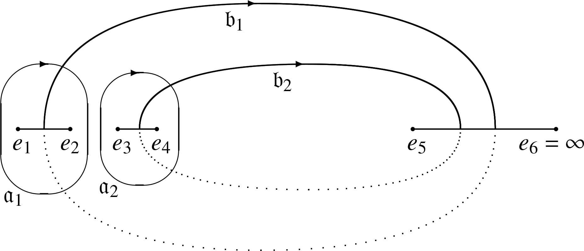
For genus-2-curves, there are 16 characteristics. 6 of them are odd and 10 even and we denote the sets of characteristics as 𝒮6 and 𝒮10, correspondingly. Odd characteristics are in 1 – 1 correspondence with the branching points, (0, 1, a1, a2, a3, ∞), in a way which will become clear in the subsequent sections.
Rosenhain’s central theorem is taken from his only known publicationa, where it was indeed unproven. We, too, give it here without proof:
Theorem 1.1 (Rosenhain’s modular representation of the period matrix 𝒜).
In the homology basis given on Fig. 1, there are characteristics
This formula was proven by H. Weber [19] during his course of deriving special case solutions of the Clebsh problem on the motion of a rigid body in an ideal liquid (see also the discussion by O.Bolza in his dissertation devoted to the reduction of genus-2 holomorphic integrals to elliptic integrals, [3], a shorter version was published in [4]).
In more recent times, the problem of a θ-constant representation of 𝒜 was discussed within NovikovŠs program of Şeffectivization of finite-gap integration formulaeŤ, see e.g. Dubrovin [5]. E.Belokolos and V.Enolskii [2] implemented this representation in their approach to the reduction of θ-functional solutions of completely integrable equations to elliptic functions. Nart and Ritzenthaler ([14]) used a Thomae-type formula for non-hyperelliptic genus-3 curves, derived from Weber’s formula ([18] and more recently [11]), but did not apply the found θ-constants to the problem of representation of 𝒜. An attempt of a generalization of Rosenhain’s work can be found in [16] and below in the Corollary 2.1.
Some of the build-up of this work can also be found in [7], in especially the recovery of Rosenhain’s formula by Thomae’s second formula. Indeed, it was V. Enolskii, who brought the topic to our attention, and we believe to have generalized their previous contributions.
Below, one of our goals is to elucidate the role that these specific characteristics play in Rosenhain’s formula. For that purpose, the next section is dedicated to the first and second Thomae Formulae in higher genera. In the 3rd section we go on with the attempt to express the period matrix 𝒜 solely by θ-constants, which will then be completed exemplarily in the 4th and 5th section for genus 2 and 3 and in doing so we will broader the class of characteristics which fulfill eq. (1.6) and its higher-genus analogues.
We believe our results will be of general interest as both for theory and for numerical calculations of complete hyperelliptic integrals.
2. Thomae formulae for hyperelliptic curves
The seminal paper from Thomae [Tho870] is mostly known for the formula relating branching points to even θ-constants of a genus-g hyperelliptic curve C. But the paper also contains a formula for non-singular derivated odd θ-constants without a proof. In this section we give an elementary proof.
2.1. Curve and differentials
Let the curve C be of the form
Fix a basis of holombrphic differentials du(P) = (du1(P), …, dug(P))T,
The normalised holomorphic differentials dv(P) = (dv1(P), …, dvg(P))T are defined as
The vectors ε and ε′ combine to a 2 × g matrix named the characteristic [ε] of the point v. If v is a half-period then all entries of the characteristic are equal 0 or 1 modulo 2.
2.2. Theta-functions
Next we introduce in greater detail the Riemann-θ-function θ[ε](z; τ), z ∈ ℂg, τ ∈ 𝔖g
It possesses the periodicity property
The property (2.7) implies
Therefore θ[ε](z; τ) is even if ε′ εT is even and odd otherwise. The corresponding characteristic is called even or odd. Among 4g characteristics there are (4g + 2g) / 2 even and (4g−2g) / 2 odd.
Following the notion of Krazer [13], p.283, a triplet of characteristics [ε1], [ε2], [ε3] is called azygetic if
The values θ[ε](0; τ) = θ[ε] are called θ-constants. An even characteristic [ε] is non-singular if θ[ε] ≠ 0, an odd characteristic [δ] is called non-singular if the derivative θ-constants,
As it is implied in eq. (2.5) we can identify any branching point ei of the curve C with a half-period,
Proposition 2.1.
[FK980] The homology basis (a, b) is completely defined by the characteristics [𝔄j], j = 1, …, 2g + 2. g of these characteristics are odd and the remaining g + 2 are even. The vector of Riemann constants
Proposition 2.2.
Let the 2g + 2 characteristics [𝔄j] be ordered into a sequence, for which the first g characteristics are odd and the remaining are even. Then such a system of characteristics is a special fundamental system.
Proof. In the light of Proposition 2.1, it is clear that there are g odd and g + 2 even characteristics. Now, the first part of the exponent of eq. (2.9) is 0 mod 2 if none or two of the three characteristics are odd, and it equals 1 mod 2 if one or three characteristics are odd. The second part of the exponent asks for the parity of a sum of three characteristics. If none or two of them are odd, the sum is odd and hence the said part of the exponent is 1 mod 2. If one or three characteristics are odd, the sum is even and the second part of the exponent is 0 mod 2. In total, the exponent is always odd and hence any triple is azygetic.
Fay ([9], p. 13) describes a one-to-one correspondence between the characteristics [ε] and the partitions of indices of branching points {1,…, 2g + 2},
Clearly, the following notation for characteristics is useful:
m is called the index of speciality of the branching point divisor and we will be interested in the cases m = 0, that deals with even non-singular θ-constants, and m = 1, the case of non-singular odd θ-constants. Here, we are considering hyperelliptic curves with a branching point at ∞ and we fix in what follows P0 = ∞. The defined sets can be written as
From the set ℐ0 2g sets ℐ1 and 𝒥1 can be defined:
It is convenient to denote the Vandermonde determinants,
2.3. Thomae theorems
We are now in the position of having set up our notation. The odd curve C will be realized as:
C has a branching point at infinity,
The next theorem is one of the key points of [17] and its proof is well-documented in the literature (e.g. [9]):
Theorem 2.1 (First Thomae theorem).
Let ℐ0 ∪ 𝒥0 be a partition of the set of indices of the finite branching points and [ε(ℐ0)] the corresponding characteristic. Then
To find ϵ, which does not depend on τ but rather on the ordering of the branching points in ∇(ℐ0), the classical way is to use a diagonal period matrix τ and use Jacobi’s θ-constants relation on the separated equations. However, we believe the quickest way to determine ϵ is to compute the θ-constants at a very low precision.
There are various corollaries of the Thomae formula (2.17). The following two are easy to prove. Their formulation is taken from [7], but the first one is also topic in [16].
Corollary 2.1.
Let 𝒮 = {n1, …, ng−1} and 𝒯 = {m1, …, mg−1} be two disjoint sets of non-coinciding integers taken from the set 𝒢 of indices of the finite branching points. Then for any two k ≠ l from the set 𝒢 \ (𝒮 ∪ 𝒯) the following formula is valid
Corollary 2.2.
Let ℐ0 = {i1, …, ig} and 𝒥0 = {j1, … jg + 1} be a partition of 𝒢. Choose k, n ∈ I0 and i, j ∈ 𝒥0 and define the sets 𝒮k = ℐ0 \ {k}, 𝒮k, n = ℐ0 \ {k, n}, 𝒯i,j = 𝒥0 \ {i, j}. Then
One can assure oneself of the correctness of these corollaries by a straightforward calculation and use of Thomaes first theorem.
Thomae’s paper contains also an important theorem describing non-singular derivated odd θ-constants. It is this, which is most significant for the course of the paper at hand:
Theorem 2.2 (Second Thomae theorem).
Let
We give here an elementary proof of this theorem. For this we first examine a helpful lemma.
Lemma 2.1.
Let 𝔄k be the Abelian image of the branching point ek and [𝔄k] its characteristic. Let
Proof. Consider the expression
As the function of
To find the constant c we use (2.17). Therefore we fix v at some branching points
Proof of Theorem 2.2.
Coming back to the proof of Theorem 2.2 we introduce the functions
First, we use these functions to compute the Jacobian
Aside from that, we compute the derivative of eq. (2.21):
To write this relation for θ-constants, we proceed like in the previous proof and fix v at certain branching points: xj = el, j = 1,…, g, l = 1,…, 2g + 1. Again we can adopt the ε-notation and write:
However, on the right hand side of eq. (2.29) all remaining yi cancel and the residual zeros of
Plugging all this together, we get:
On
Example: The genus-1 case
Let C be the Weierstrass cubic,
In this case we have:
Using further [1], vol 3, Sect 13.20
Example: The genus-g case
With much the same method, one can obtain a generalization of eq. (2.32) to arbitrary genus, which is known as the Riemann-Jacobi-formula (for hyperelliptic curves). For that to formulate we introduce the g + 1 sets
Further, we need the Jacobi matrix J:
Then, the following relation is valid:
This is a long-known result and part of a more general Riemann-Jacobi formula, see e.g. [12] for a modern outline, or [10]. The formulation used here is at least valid for θ-functions with a given hyperelliptic curve in a fixed homology basis, see [7] for a check within the methods described here. There, we find also a useful matrix notation for the second Thomae formula, which we will adopt in the next section:
2.4. Matrix form of the Second Thomae formula
The formula (2.20) can be written in matrix form. With all the definitions above, one immediately recognises that this comes to:
This formula can also be rewritten as
This can be treated further. To do that we write our given curve of genus g (with a branching point at infinity) in the form:
After inverting eq. (2.38), we get:
Next, we want to use the Riemann-Jacobi formula on det J. For that we need the g + 1 sets 𝒯k = 𝒥0 \ {jk}, so that we can write:
Note, that 𝒯0 is excluded from the product, which will be useful later, as well as the label of Θ. We can process θ[ε(𝒯0)] further with the help of the first Thomae theorem, so that most of the prefactors cancel and only a ∇1 / 4(ℐ0) remains in the denominator. As
Of course, one can consider also the not-inverted, original period matrix 𝒜, and using the same steps on 𝒟 as before, we can rewrite eq. (2.38) as:
But we decided to work primarily on the inverted matrix, because this is, what Rosenhain’s formula gives us. Another advantage is that we can quickly recover and generalize Bolza’s formula. For that purpose we write our result in the following way:
Proposition 2.3.
Let C be a hyperelliptic curve of genus g with one branching point at infinity. Let ℐ0 ∪ 𝒥0 = {i1,…,ig} ∪ {j1, …, jg + 1} be a partition of 2g + 1 indices of branching points. Then the columns Um of the matrix 𝒜−1 are of the form
2.5. Bolza formulae
Let
For a genus-2 curve with branching points e1,…, e2g + 1, Bolza ([4]) found that
Enolskii et al. reproved and generalized this formula in [6] by using Kleinian σ-functions. With the help of eq. (2.48) we can find a quicker proof and write it in a concise way:
As we have done before, we choose P0 = ∞ and keep the notation of ε instead of 𝔄. For a general hyperelliptic curve of genus g we consider the expression
There are g different sets
Corollary 2.3.
Let
Example: genus 3
Take ℐ0 = {1,2,3} and hence
3. A general θ-constant form of 𝒜−1
Though eq. (2.48) gives us a good tool, our final goal is to completely express 𝒜−1 with θ-constants for those cases where only τ is known. Thus, we want to work more on χk. We can achieve that by the use of eq. (2.21).
Theorem 3.1.
Let ℐ0 = {n, i1, …, ig−1} and 𝒥0 = {j1, …, jg + 1} be a partition of branching points, such that y2 = ϕ(x) ψ(x) with
Let further ℐ1 = ℐ0 \ {n}. For
Proof. Take eq. (2.21) and evaluate v at the branching points
Squaring this and iterating the procedure for every left-over jg + 1 we get:
This equality comes from the fact that there are g times g + 1 terms in the numerator and every linear factor occurs g times, but is canceled once by the denominator. The residual parts fit the definition of 𝛘n.
Finally, we recognize ε({n} ∪ 𝒥0 \ {j} = ε({n} ∪ ℐ0 ∪ {j}) = ε(ℐ1 ∪ {j}) to arrive at the definition of
Note: In eq. (3.2) are as much factors in the numerator as in the denominator. Therefore, we can interchange the ordering of the en and ej without changing the global prefactor ϵ, if one simultaneously changes the ordering of the en and ei in the denominator.
4. Genus 2: Recovery of Rosenhain’s formula
4.1. The Rosenhain derivatives
Consider the case g = 2 and the curve given as
In the homology basis drawn on Fig. 1 we have
The characteristic of the vector of Riemann constants reads
The characteristics in question here are:
One also has to hold in mind, that the sum of all characteristics Ai is zero, so that 2-indexed ε and 3-indexed ε can be interchanged (as shown for instance in eq. (4.3)).
We are now in the position to exemplary investigate the sets 𝒯l of eq. (2.33) and henceforward
The already defined quantity
This choice of the sets leads us directly to the following Rosenhain derivative formula as a consequence of the Riemann-Jacobi-formula:
In general, for the different choices of εi, εj as odd characteristics Riemann-Jacobi gives us
For any triple {i, j, k} ⊂{1,…, 6} we can regard the three Rosenhain derivative formulae belonging to the sets
Here, Θ{i, j} = θ[εklp]θ[εkmp]θ[εklm], as it is apparent from the construction. 3-indexed ε can be changed to 2-indexed ε if convenient. Each two of eq. (4.7) can be used to solve for θn[εi], θn[εj] or θn[εk], n = 1, 2, and the third one provides a useful substitution. In the course, εlmp cancels and we arrive at the following lemma:
Lemma 4.1.
For any odd genus-2 curve C and one from 20 triples {i, j, k} ⊂{1, …, 6} (with.ε6 ≡ K∞) the following relation holds:
For the choice above, ℐ0 = {1,2}, we deliberately pick as the third index 6. Eq. (4.8) gives us:
For other partitions one has to keep in mind the sign in eq. (4.8) and switch the order of the characteristics if required.
4.2. General Rosenhain Theorem
With our chosen partitions eq. (2.46) reads
Theorem 3.1 gives us:
To compare this result with the Rosenhain-memoir [15] we apply a Moebius transformation to the curve, which sets e1 = 0 and e2 = 1. Now using Θ{1,2}, Θ{1,6} and Θ{2,6} as well as eq. (4.9) we find:
We now can identify δ1 = ε1, δ2 = K∞, P = Θ{2,6} and Q = Θ{1,2} and hence we have recovered Rosenhain’s theorem, eq. (1.6), along with the extra identity
We used here the partition {1, 2} ∪ {3, 4, 5} in order to compare it to Rosenhain’s original theorem. But the techniques of Theorem 3.1 and Lemma 4.1 allow for a more general statement:
We take the sets ℐ0 = {i, j} and 𝒥0 = {k, l, m}, all indices mutually disjoint. Again, we normalize the curve to ei = 0 and ej = 1 by means of a Moebius transformation.
One can see, that for a set ℐ0 = {i, j} it is always necessary to pick 6 as the third index for Lemma 4.1 to be applicable in this context. We arrive at the following theorem:
Theorem 4.1 (General genus-2 Rosenhain Theorem).
For an odd genus-2 curve C with normalized branching points ei = 0, ej = 1 and arbitrary branching points ek, el, em the inverse period matrix 𝒜−1 is given as:
In the same fashion one can indicate 𝒜 if desired. We therefore invert eq. (4.13) using eq. (4.7) one time. We conclude:
Note that this formula incorporates all 10 even characteristics. Also, the three characteristics in Θ{i, j} sum up to (the odd) K∞ and the three characteristics in Θ{j, 6} sum up to (the odd) εi.
5. A genus-3 Rosenhain formula
We take a hyperellipticc curve in the form,
The characteristics of the Abelian images of branching points are
The vector of Riemann constants K∞ with base point at P8 = ∞ is given in this homology basis as
The important characteristics are here:
The Riemann-Jacobi formula for this choice of ℐ0 (and hence 𝒥0 = 𝒯0 = {4, 5, 6, 7}) reads
Following the necessary steps, eq. (2.48) gives us for 𝒜−1 = (U1, U2, U3):
If required, we could use eq. (2.47) to arrive at 𝒜. But currently we see no further simplifications and therefore didn’t depict it here.
6. Concluding remarks
Without any major changes, one can adopt the method shown for genus 3 to higher genera. Unfortunately we were not able to find a generalization to Lemma 4.1, which could bring eq. (5.7) down to a structure like in eq. (1.6). It seems unlikely that there exists one as simple as in genus 2.
Our next steps in this work could be to unfix the base point, which was infinity throughout this work. And we see a chance to develop Thomae type formulae expressing higher derivative θ-constants. We hope to come back to this topic in the near future.
Acknowledgments
The author wants to thank Victor Enolskii and Chris Eilbeck for providing the idea of the work and many suggestions for useful techniques as well as the constant interest in the work. Also the author gratefully acknowledges the Deutsche Forschungsgemeinschaft (DFG) for financial support within the framework of the DFG Research Training group 1620 Models of gravity.
Appendix A. Rosenhain derivative formulae
For any two odd characteristics [δ1], [δ2] denote
Then the following 15 Rosenhain derivative formulae are valid
We pointed at the right margin the characteristic, which is the sum of characteristics of each entry to the corresponding equality.
Footnotes
Wikipedia tells us: “Rosenhain galt auch als begabt in Sprachen und Musik; allerdings bemerkten einige Beobachter, dass er die hohen Erwartungen seiner jungen Jahre nicht erfüllte und nach seiner preisgekrönten Arbeit keine nennenswerten Beiträge mehr veröffentlichte.”
This case generically occurs in our method if one chooses the partition I (see below) strictly even or odd with respect to the characteristics.
If not stated otherwise we always mean hyperelliptic curves.
References
Cite this article
TY  - JOUR
AU  - Keno Eilers
PY  - 2021
DA  - 2021/01/06
TI  - Rosenhain-Thomae formulae for higher genera hyperelliptic curves
JO  - Journal of Nonlinear Mathematical Physics
SP  - 86
EP  - 105
VL  - 25
IS  - 1
SN  - 1776-0852
UR  - https://doi.org/10.1080/14029251.2018.1440744
DO  - 10.1080/14029251.2018.1440744
ID  - Eilers2021
ER  -