Journal of Nonlinear Mathematical Physics

Volume 25, Issue 2, March 2018, Pages 211 - 246

Symmetry Reduction of Ordinary Differential Equations Using Moving Frames

Authors
Francis Valiquette
Department of Mathematics, State University of New York at New Paltz, 1 Hawk Drive, New Paltz, NY 12561, USA,valiquef@newpaltz.edu
Received 27 March 2017, Accepted 29 November 2017, Available Online 6 January 2021.
DOI
10.1080/14029251.2018.1452671How to use a DOI?
Keywords
Canonical variables; differential invariants; equivariant moving frames; Lie point symmetries; ordinary differential equations
Abstract

The symmetry reduction algorithm for ordinary differential equations due to Sophus Lie is revisited using the method of equivariant moving frames. Using the recurrence formulas provided by the theory of equivariant moving frames, computations are performed symbolically without relying on the coordinate expressions for the canonical variables and the differential invariants occurring in Lie’s original procedure.

Copyright
© 2018 The Authors. Published by Atlantis and Taylor & Francis
Open Access
This is an open access article distributed under the CC BY-NC 4.0 license (http://creativecommons.org/licenses/by-nc/4.0/).

1. Introduction

Lie group integration techniques are amongst the most effective methods available for obtaining analytic solutions of nonlinear differential equations. Nowadays, there are many excellent textbooks surveying the subject, [3,58,10,1517,27,3537]. Following Sophus Lie’s seminal ideas, most symmetry-based integration methods rely on the infinitesimal symmetry generators of the differential equation under consideration. For example, given an nth order ordinary differential equation with one infinitesimal symmetry generator, there is a well known procedure for reducing the order of the equation by one by introducing canonical variables that rectify the infinitesimal symmetry generator. More generally, if the differential equation admits an r-dimensional solvable symmetry group, then the equation can be reduced to an order nr differential equation, assuming n > r. Given a solution to the reduced equation, the solution to the original differential equation can then be recovered by quadrature.

To find the canonical variables (t, s) that rectify an infinitesimal symmetry generator, a system of first order linear partial differential equations must be solved. Once the canonical variables have been found, the order of the differential equation is reduced by re-expressing the equation in those new coordinates and introducing the new dependent variable w = st. For r-dimensional solvable symmetry groups, this procedure is repeated r times. At each iteration, one must keep track of the coordinate expressions of the prolonged infinitesimal symmetry generators in the new system of coordinates in order to compute the subsequent set of canonical variables to be introduced in the following iterations. For large symmetry groups, these coordinate dependent computations can become cumbersome and thereby limit the scope of the method. The main goal of the present paper is to present a symbolic implementation of Lie’s symmetry reduction procedure for ordinary differential equations that does not rely on the coordinate expressions of the canonical variables and the differential invariants occurring in the standard implementation of the method. The constructions introduced are completely algorithmic and can therefore directly be implemented in symbolic computer packages such as Maple, Mathematica, or Sage.

This paper is part of recent efforts aimed at developing new symbolic computational tools for differential equations based on the method of equivariant moving frames. Recent developments have occurred in the calculus of variations, [19,38], the computation of conservation laws, [1214], the theory of geometric curve flows, [4,23,24,29], the classification of differential invariants and their syzygies, [9,33], the symmetry classification problem of differential equations, [21], the general equivalence problem of differential equations, [25,41], and the method of group foliation, [22,39]. For a comprehensive overview of modern applications of the method of equivariant moving frames, we refer the reader to [22,31].

For one-dimensional symmetry groups, our symbolic implementation of the symmetry reduction algorithm is based on the standard implementation of the equivariant moving frame method, [11,22]. For solvable symmetry groups, we use the inductive/recursive moving frame constructions introduced in [18,30,34,40] as group parameters are recursively normalized each time the order of the differential equation is reduced. As a byproduct, the ideas developed in this paper provide a new and nontrivial application of the inductive and recursive moving frame implementations introduced in [18,30,34,40]. When compared to the group foliation method developed in [22,39], where group parameters are normalized all at once, the recursive approach proposed in this paper offers several benefits. Firstly, as illustrated in [15], it is possible that one of the intermediate equations obtained during the reduction process is easier to solve than the final reduced equation. This situation can occur if, for example, one of the intermediate equations admits (type II) hidden symmetries, [1,20]. In this case, since the group foliation method only computes the final reduced equation, it would miss the intermediate reduced equation that allows to solve the original differential equation more easily. Secondly, in the implementation of the group foliation method, it is not clear which normalizations will produce the simplest reduced equation. On the other hand, when group parameters are normalized recursively, the reduced equation obtained at each stage of the symmetry reduction process can help make educated normalizations that will lead to the simplest reduced differential equation. Finally, in contrast to the group foliation method introduced in [22], our approach does not require the introduction of a “computational variable” when the independent variable is not an invariant of the group action. Avoiding the introduction of computational variables is generally desirable as these tend to lead to more complicated differential equations and also require the introduction of a “companion equation”, which leads to the problem of solving a system of differential equations rather than just the original equation.

Given the solution to the fully reduced differential equation, we introduce a recursive reconstruction procedure for recovering the solution to the original differential equation. As in the reduction step, the reconstruction computations are performed symbolically without requiring coordinate expressions for the invariants introduced during the reduction process. To implement the reconstruction procedure, the main data required is the induced action of the various one-parameter groups on the invariants at each step of the reduction process. As it will be shown in Section 5.2, these one-parameter group actions (more precisely their corresponding infinitesimal generators a) can be deduced symbolically using the recurrence relations provided by the theory of equivariant moving frames, [11,19,32].

For completeness, we begin in Section 2 by recalling standard notation and basic definitions pertaining to ordinary differential equations and symmetry groups. Lie’s symmetry reduction algorithm for ordinary differential equations is then reviewed in Section 3, and the basic equivariant moving frame constructions are laid out in Section 4.1. In particular, the recurrence formulas for the normalized differential invariants are introduced. These equations provide a complete characterization of the structure of the algebra of differential invariants and their syzygies. An important aspect of these equations is that they can be obtained symbolically without relying on the coordinate formulas of the differential invariants or the moving frame. In Section 4.2, the inductive/recursive implementation of the moving frame method is introduced. Using the method of moving frames, Lie’s symmetry reduction algorithm for one-dimensional symmetry groups is revisited in Section 5.1, and the general case for solvable symmetry groups is considered in Section 5.2.

2. Preliminaries

Let J(n)=Jn(,) denote the nth order jet bundle of smooth maps u:. In the following, we allow the domain of the function u(x) to be an open subset of . Local coordinates on J(n) are given by (x, u(n)), where x denotes the independent variable and u(n) = (u, ux, uxx,…,un) collects the derivatives of the dependent variable u, up to order n. A basis of one-forms on the infinite-order jet bundle J(∞) is given by the horizontal one-form dx and the basic contact forms

θk=dukuk+1dx,k0.(2.1)
This decomposition splits the exterior derivative into horizontal and vertical (or contact) components, and endows the space of differential forms on J(∞) with the structure of a variational bicomplex, [2,19,38]. The contact forms (2.1) play a fundamental role in the calculus of variations, but for the purpose of this paper these can be omitted. For this reason, all our considerations are done modulo contact forms.

Definition 2.1.

An nth order ordinary differential equation is the zero locus of a differential function Δ:J(n):

Δ(x,u(n))=0.(2.2)

Definition 2.2.

An ordinary differential equation Δ(x,u(n)) = 0 is said to be regular if its differential dΔ ≠ 0 does not vanish on the domain of definition of the equation. A differential equation is locally solvable at the point (x0,u0(n)) if Δ(x0,u0(n))=0 and there exists a smooth solution u = f(x), defined in the neighborhood of x0, such that u0(n)=f(n)(x0). An ordinary differential equation which is both regular and locally solvable is said to be fully regular.

In the following, we only consider fully regular ordinary differential equations. Now, let

v=ξ(x,u)x+φ(x,u)u(2.3)
be a local vector field on J(0)2. The flow of the vector field (2.3) induces the one-parameter group of local transformations
(X,U)=gε(x,u)=exp[εv](x,u),ε.(2.4)
The corresponding one-parameter Lie group is denoted by Gε. We observe that Gε is locally isomorphic to the Lie group (,+). In turn, the one-parameter group action (2.4) induces an action on the nth order jet bundle J(n), called the nth order prolonged action, [27]. To obtain the coordinate expressions of the prolonged action, we introduce the implicit derivative operator
DX=1DxXDx=1Xx+XuuxDx,(2.5)
where
Dx=x+k=0uk+1uk
is the total derivative operator with respect to the independent variable x. The nth order prolonged action is then obtained by successively differentiating U = gεu with respect to the implicit derivative operator (2.5):
UXk=gεuxk=DXk(U),k=1,,n.(2.6)
At the infinitesimal level, the nth order prolongation of the infinitesimal generator (2.3) is given by the vector field
v(n)=ξ(x,u)+k=0nφk(x,u(k))uk,
where the coefficient φk(x, u(k)) is defined recursively by the formula
φk+1=Dxφkuk+1Dxξ.

Definition 2.3.

A one-parameter Lie group Gε is said to be a symmetry group of the fully regular ordinary differential equation (2.2) if for every gεGε

Δ(gε(x,u(n)))=0 whenever Δ(x,u(n))=0.
At the infinitesimal level, equation (2.2) is invariant if for all infinitesimal generator v in the Lie algebra g of Gε, we have
v(n)(Δ)=0 whenever Δ=0.

Remark 2.1.

The above exposition easily extends to systems of ordinary differential equations involving several dependent variables u = (u1,…,uq). Also, the one-parameter group Gε in Definition 2.3 can, in general, be replaced by an r-dimensional Lie group G.

3. Symmetry Reduction

We now review Lie’s symmetry reduction algorithm for an ordinary differential equation invariant under a one-parameter symmetry group, [3,58,10,1517,27,3537]. Therefore, let Δ(x,u(n)) = 0 be an ordinary differential equation invariant under the infinitesimal symmetry generator (2.3). The standard symmetry reduction algorithm is based on the introduction of a set of canonical variables

(t,s)=Φ(x,u)(3.1)
in which the vector field (2.3) takes the rectified form
v=s.(3.2)
The canonical coordinates (t, s) are found by solving the system of linear first order partial differential equations
v(t)=ξtx+φtu=0,v(s)=ξsx+φsu=1,(3.3)
using the method of characteristics. Letting s be the dependent variable and t the independent variable, the differential equation Δ(x, u(n)) = 0 can be rewritten in these new coordinates:
Δ˜(t,s(n))=Δ(x,u(n))=0.
Since equation Δ˜(t,s(n))=0 is invariant under the infinitesimal symmetry generator (3.2), the equation must be independent of s:
Δ˜(t,s(n))=Δ˜(t,st,stt,,stn).
Introducing the new dependent variable w = st, the order of the differential equation is decreased by one:
Δ˜(t,w,wt,,wtn1)=Δ˜(t,w(n1))=0.(3.4)

Assuming w = w(t) is the general solution of the reduced equation (3.4), we have that

s(t)=w(t)dt,
and that the solution to the original differential equation Δ(x, u(n)) = 0 is obtained by inverting the change of variables (3.1):
(x(t),u(t))=Φ1(t,s(t)).
The latter gives a parametrized solution with parameter t. Expressing t = t(x) as a function of x, the solution to the original differential equation Δ(x, u(n)) = 0 is u(t(x)).

As it is well known, the above reduction procedure can be iterated for multi-parameter solvable symmetry groups. Since there are different, yet equivalent, definitions of solvable Lie groups, we now introduce the definition used in the paper, which can be found in [27].

Definition 3.1.

Let G be an r-dimensional Lie group with Lie algebra g. The Lie group G is said to be solvable if there exists a chain of Lie subgroups

{e}=G(0)G(1)G(2)G(r1)G(r)=G(3.5)
such that for each = 1, . . . , r, G() is a -dimensional subgroup of G and G( − 1) is a normal subgroup of G(). At the infinitesimal level, the Lie algebra g is solvable if there exists a chain of Lie subalgebras
{0}=g(0)g(1)g(2)g(r1)g(r)=g,(3.6)
such that for each , dimg()= and g(1) is a normal subalgebrab of g(), which means that
[g(1),g()]g(1).

Assuming Δ(x, u(n)) = 0 is invariant under an r-dimensional solvable symmetry group G, the solvable structure of the symmetry group G will dictate the order in which symmetry reduction should by performed. After the introduction of a convenient basis { v1,…vr} for g, assume that

g()=span{v1,,v},=1,,r.(3.7)
Such a set of vectors is said to form a canonical basis, [15] According to this canonical basis, the differential equation Δ(x, u(n)) = 0 is first reduced using the infinitesimal generator v1. The resulting equation is then reduced using v2, v3, and so on up to vr. At the th  iteration, the solvable structure of the symmetry group guarantees that the resulting reduced equation is invariant under the infinitesimal symmetry generators v+1,,vr.

The overall process can be computationally demanding as each time the order is reduced, new canonical variables are computed and the prolonged infinitesimal symmetry generators have to be re-expressed in these new coordinates. In Section 5, we will show how these coordinate dependent computations can be avoided using the method of moving frames. But before doing so, we illustrate Lie’s symmetry reduction algorithm with a simple example. This will allow us to compare the standard implementation to the moving frame implementation introduced in Section 5.

Example 3.1.

To illustrate Lie’s symmetry reduction procedure, we consider the second order ordinary differential equation

x2uxx=F(xuxu),(3.8)
where, for now, F: is an arbitrary function. Equation (3.8) admits a two-dimensional symmetry Lie algebra spanned by the vector fields
v1=xu and v2=xx.(3.9)
The commutator of these two vector fields is
[v1,v2]=v1.
The Lie algeba is therefore solvable c with the chain of normal subalgebras
{0}g(1)=span{v1}span{v1,v2}=g.
We therefore start implementing the symmetry reduction algorithm using the infinitesimal generator v1. The canonical variables (t, s) are found by requiring that
v1(t)=xtu=0,v1(s)=xsu=1.(3.10)
Using the method of characteristics, a solution is given by
t=x,s=ux.(3.11)
In these new variables, equation (3.8) becomes
t3stt+2t2st=F(t2st).
Introducing the new dependent variable w = st, we obtain the first order reduced differential equation
t3wt+2t2w=F(t2w).(3.12)

Expressing the first order prolonged infinitesimal generator

v2(1)=xxuxux
in the variables
t=xs=ux,w=st=xuxux2,
we find that
v2(1)=ss+tt2ww.
Therefore, v2(1) has a well-defined restriction to the invariants (t, w):
v^2=v2(1)|(t,w)=tt2ww.
Now let (y, z) be new canonical variables that rectify v^2 to z. These variables are found by solving the system of linear partial differential equations
v^2(y)=tyt2wyw=0,v^2(z)=tzt2wzw=1.
A solution to these equations is given by
y=t2w,z=lnt.(3.13)
In those variables
zy=12t2w+t3wt,
and the differential equation (3.12) becomes
zy=1F(y).
To integrate the latter equation explicitly, one has to consider a particular function F(y). For example, if F(y) = y2 then
zy=1y2 and z(y)=1ylnC.(3.14)
Substituting (3.13) into (3.14) we get
lnt=1t2wlnC, which implies that w=1t2ln(Ct).
Recalling that w = st, we have
s(t)=w(t)dt=CE1(ln(Ct))+K,
where E1(x) = − Ei( − x) and Ei(x) is the exponential integral function, [26]. Substituting (3.11) into the latter result yields
u(x)=CxE1(ln(Cx))+Kx,
which is the general solution to the nonlinear differential equation
x2uxx=(xuxu)2.(3.15)

4. Moving Frames

We now introduce the moving frame constructions that will be used in the symbolic implementation of the symmetry reduction process introduced in Section 5. In Section 4.1, we first survey the standard implementation of the equivariant moving frame method as originally introduced in [11]. In Section 4.2, we review the inductive/recursive implementation of the moving frame method developed in [18,30,34,40].

4.1. Standard implementation

Let G be an r-dimensional Lie group acting smoothly on the nth order jet space J(n). A right moving frame is a G-equivariant map ρ: J(n)G, where G-equivariance means that

ρ(g(x,u(n)))=ρ(x,u(n))g1
for all gG where the prolonged action and the moving frame are defined. To every right moving frame ρ corresponds a left moving frame ρ¯ given by group inversion:
ρ¯(x,u(n))=(ρ(x,u(n)))1.

The main existence theorem states that a moving frame exists in the neighborhood of a point (x, u(n)) ∈ J(n) provided the action is (locally) free and regular on that neighborhood. We recall that the action is free at a point (x, u(n)) if the isotropy group

G(x,u(n))={gGg(x,u(n))=(x,u(n))}={e}
is trivial, and that the action is locally free at a point if the isotropy group is discrete. The action is regular if the group orbits have the same dimension and each point (x, u(n)) ∈ J(n) has arbitrary small neighborhoods whose intersection with each orbit is a connected subset thereof. A theorem originally due to Ovsiannikov, [35], and then corrected by Olver, [28], guarantees that any finite-dimensional Lie group acting locally effectively on subsets of J(0)2 will eventually act locally freely on an open dense subset of J(n) for a sufficiently large n. Therefore, a moving frame will exist provided the action is prolonged to a sufficiently high order jet space.

The construction of a moving frame is based on the introduction of a cross-section KJ(n) to the group orbits. By definition, a cross-section K is a submanifold transverse and of complementary dimension to the group orbits. In general, it is specified by a system of r = dimG equations

K={F(x,u(n))=0=1,,r}.
To simplify the discussion, we assume
K={z1=c1,,zr=cr}J(n)(4.1)
is a coordinate cross-section obtained by setting r coordinates of the n-jet (x, u(n)) to constant values. The right moving frame ρ(x, u(n)) ∈ G at (x, u(n)) is then the unique group element that sends (x, u(n)) onto the cross-section K:
ρ(x,u(n))(x,u(n))K.
Coordinate expressions for the moving frame are obtained by solving the normalization equations
Z=gz=c,=1,,r,
for the group parameters g = (g1,…,gr).

Example 4.1.

To illustrate the moving frame construction, we consider the two-parameter group action

X=eε2x,U=u+ε1x,ε1,ε2,(4.2)
acting on the right half-plane +×. To compute the induced prolonged action, we introduce the implicit derivative operator
DX=1eε2Dx.(4.3)
Applying (4.3) to U = u + ε1x, we obtain, up to order two, the prolonged action
UX=DX(U)=ux+ε1eε2,UXX=DX(UX)=uxxe2ε2.
Choosing the coordinate cross-section
K={x=1,u=0},
and solving the normalization equations
1=X=eε2x,0=U=u+ε1x,(4.4)
for the group parameters (ε1, ε2), we obtain the right moving frame
ρ(x,u):ε1=ux,ε2=ln1x.(4.5)

To proceed further, we introduce the nth order lifted bundle G(n)=J(n)×G. The Lie group G acts on G(n) by the lifted action

g((x,u(n)),h)=(g(x,u(n)),hg1),(4.6)
also known as the anti-diagonal action of G on G(n).

Definition 4.1.

The lift of a differential function F:J(n) to the lifted bundle G(n) is defined as

λ[F(x,u(n))]=F(g(x,u(n))),(4.7)

We observe that the lifted function (4.7) is invariant under the lifted action (4.6). We therefore refer to (4.7) as a lifted invariant. In particular, lifting the jet coordinates (x, u(n)):

λ(x,u(n))=g(x,u(n))=(X,U(n)),
we recover the prolonged action (2.6). The quantities (X, U(n)) are called fundamental lifted invariants. This terminology is motivated by the fact that any lifted invariant is a function of the fundamental lifted invariants:
λ[F(x,u(n))]=F(λ(x,u(n)))=F(X,U(n)).
Inversely, given a lifted invariant F(X, U(n)), we introduce the inverse lift
λ1[F(X,U(n))]=F(x,u(n)),
which is defined as the function whose lift is F(X, U(n)).

The lift map λ extends to differential forms, and we refer to [11] for more detail. For the purpose of this paper, it is enough to know that, modulo the contact forms (2.1), the lift of the horizontal form dx is

ω=λ(dx)=Dx(X)dx=(Xx+Xuux)dx.

Given a right moving frame ρ: J(n)G, we introduce the right moving frame section ϱ:J(n)G(n) defined as

ϱ(x,u(n))=((x,u(n)),ρ(x,u(n))).

Definition 4.2.

Let ρ: J(n)G be a right moving frame. The invariantization map is defined as

l=ϱ*λ.

Invariantizing a differential function F:J(n), we obtain the differential invariant

ı(F)(x,u(n))=F(ρ(x,u(n))(x,u(n))).(4.8)
The fact that (4.8) is a differential invariant follows from the G-equivariance of the right moving frame ρ(x, u(n)). Of particular importance is the invariantization of the jet coordinates (x, u(n)). The differential invariants
H=ı(x),I(n)=ı(u(n))(4.9)
are called normalized invariants. By construction of the right moving frame, the invariantization of the coordinates used to define the cross-section (4.1) are constants, that is
ı(z)=c.(4.10)
These normalized invariants are called phantom invariants. By the replacement principle, [11,22] the normalized invariants (4.9) form a complete set of differential invariants of order ≤ n. This means that any differential invariant of order ≤ n can be expressed in terms of the normalized invariants (4.9). Indeed, since the invariantization of an invariant J(x, u(n)) is the invariant itself,
J(x,u(n))=ı(J(x,u(n)))=J(ı(x,u(n)))=J(H,I(n)).
We also note that the normalized invariants (4.9) provide a local parametrization of the cross-section (4.1) used to construct the moving frame ρ:
K={(H,I(n))}.

The invariantization of the horizontal form dx is the contact-invariant d horizontal one-form

ϖ=ı(dx)=ϱ*λ(dx)=ϱ*(ω)=ϱ*(Xx+Xuux)dx.(4.11)

Example 4.2.

Continuing Example 4.1, the invariantization of the jet coordinates ux and uxx yields the differential invariants

I1=ı(ux)=ux+ε1eε2|(4.5)=xuxu,I2=ı(uxx)=uxxe2ε2|(4.5)=x2uxx.(4.12)
The contact-invariant horizontal one-form (4.11) is given by
ϖ=ı(dx)=1xdx.(4.13)

One of the most important results from the theory of equivariant moving frames is the introduction of the universal recurrence relations for the lift map and the invariantization map. These equations can be used to perform many computations symbolically without requiring coordinate expressions for the lifted or normalized invariants. The universal recurrence relations have played a fundamental role in the development of the group foliation method, [22,39], the theory of invariant variational bicomplexes, [19,38], the study of invariant geometric curve flows, [24], the characterization of the algebra of differential invariants, [33], the development of the recursive moving frame construction, [30,34], and many other problems in applied mathematics, [31]. In order to introduce these recurrence formulas, let

v=ξ(x,u)x+φ(x,u)ug,=1,,r,
be a basis of infinitesimal generators of the Lie group action. Dually, let μ1,,μrg*, be a basis of Maurer-Cartan forms. Modulo the contact forms (2.1), the universal recurrence formula for the lift map is
d[λ(F)]=λ[Dx(F)]ω+=1rλ[v()(F)]μ,(4.14)
where F:J(n) is an arbitrary differential function e. In particular, substituting the function F in (4.14) with the jet coordinate functions (x, u(∞)), we obtain the recurrence relations for the fundamental lifted invariants X, U(∞):
dX=ω+=1rλ(ξ)μ,dUk=Uk+1ω+=1rλ(φk)μ,k0. (4.15)
Pulling back the universal recurrence relation (4.14) by the right moving frame section ϱ, we obtain the universal recurrence relation for the invariantization map
d[ı(F)]=ı[Dx(F)]ϖ+=1rı[v()(F)]v,
where v = ρ*(μ) denotes the moving frame pull-back of the Maurer-Cartan form μ. In particular, pulling back (4.15) by the right moving frame section ϱ, we obtain the recurrence relations for the normalized invariants H = ı(x), I(∞) = ı (u(∞)):
dH=ϖ+=1rı(ξ)v,dIk=Ik+1ϖ+=1rı(φk)v,k0. (4.16)

Remark 4.1.

The lifted recurrence relations (4.15) can be computed symbolically without relying on the coordinate expressions of the lifted invariants, the lifted horizontal form ω, and the MaurerCartan forms μ1,…,μr. The only data required are the expressions for the infinitesimal generators v1, …,vr, and their prolongation. Similarly, the invariantized recurrence relations (4.16) can be computed symbolically without knowing the coordinate expressions of the right moving frame ρ(x, u(n)). Indeed, using the recurrence relations for the phantom invariants (4.10), one can solve for the normalized Maurer-Cartan forms v1,…,vr. Substituting these expressions into the remaining recurrence relations provides symbolic expressions for the differential of the non-phantom normalized invariants.

Example 4.3.

To illustrate the above considerations, we consider the group action (4.2) with infinitesimal generators (3.9). First, the recurrence relations for the lifted invariants are

dX=ω+Xμ2,dU=UXω+Xμ1,dUX=UXXω+μ1UXμ2,dUk=Uk+1ωkUkμ2,k2. (4.17)
Pulling back (4.17) by the moving frame section induced by (4.5), we obtain the invariantized recurrence relations
0=ϖ+v2,0=I1ϖ+v1,dI1=I2ϖ+v1I1v2,dIk=Ik+1ϖkIkv2,k2. (4.18)
As observed in Remark 4.1, the moving frame expressions (4.5) are not needed to deduce (4.18) Indeed, the recurrence relations (4.18) are obtained symbolically by substituting the normalizations (4.4) into (4.17) and making the substitutions UkIk,ωϖ, and μv.

Solving for the normalized Maurer-Cartan forms v1, v2 using the first two equations in (4.18) we find that

v1=I1ϖ,v2=ϖ.
Substituting these expressions into the remaining equations, we obtain the recurrence relations for the non-phantom normalized invariants:
dI1=I2ϖ,dIk=(Ik+1+kIk)ϖ,k2.(4.19)

4.2. Inductive/recursive implementation

We now review the inductive/recursive implementation of the moving frame method as introduced in [18,30,34,40]. The idea behind the inductive/recursive implementation is to take into account the existence of a smaller subgroup NG for which a moving frame and its normalized differential invariants have already been constructed, and use this information to streamline the construction of a moving frame for the larger group G and the computation of its normalized differential invariants. To this end, let NG be an s-dimensional normal Lie subgroup of the r-dimensional Lie group G. In general N does not have to be normal to implement the inductive/recursive moving frame algorithm. We make this assumption here, as this is the geometric setting in which we will apply the constructions in Section 5.

For convenience, let

g=(g1,,gs,gs+1,,gr)=(h,g^)(4.20)
be local coordinates of the Lie group G such that the first s components h = (g1, …, gs) parametrize the subgroup N. Since N is normal, the quotient group G / N is well-defined and
G/N{g^=(gs+1,,gr)}.
In the following we will make us of this isomorphism and use g^ as local coordinates on G / N.

Assuming the prolonged action of N on the nth order jet space J(n) is free and regular, let ρN : J(n)N be the right moving frame induced by the coordinate cross-section

KN={z1=c1,,zs=cs}J(n).
Also, let ıN be the induced invariantization map. With the moving frame ρN and the normalized invariants (H, I(n)) = (ıN (x), ıN (u(n))) in hand, we seek to construct the normalized invariants of the larger group G inductively. To guarantee the existence of a moving frame, we assume that the prolonged action of G on J(n) is also free and regular. Now, for any hN, we observe that
λG(x,u(n))=g(x,u(n))=(gh1)h(x,u(n))=g˜(X,U(n))=λG(X,U(n)),(4.21)
where g˜G and (X, U(n)) = λN (x, u(n)) = h · (x, u(n)) denotes the N-lifted invariants. Equation (4.21) shows that the lift of the jet coordinates (x, u(n)) with respect to the group G, which we refer to as the G-lift of (x, u(n)), is equal to the G-lift of the N-lifted invariants. Replacing the group parameter hN in (4.21) by the right moving frame ρN : J(n)N, we conclude that
λG(x,u(n))=λG(H,I(n)).(4.22)
That is, the G-lift of the jet coordinates (x, u(n)) is equal to the G-lift of the N-normalized invariants (H, I(n)). We note that in applications, since the N-phantom invariants ıN(z1)=c1,,ıN(zs)=Cs are typically set equal to 0 or ± 1, the formulas on the right-hand side of (4.22) are usually simpler than those appearing on the left-hand side. The inductive construction of the G-normalized invariants is achieved by first considering the partial normalizations
λG[ıN(z)]=λG(c)=c,=1,,s,(4.23)
obtained by requiring that the N-phantom invariants remain unchanged under the prolonged action of G. Solving the normalization equations (4.23) for the group parameters hN, we can write h in terms of g^ and the N-normalized invariants (H, I(n)) :
h=h(H,I(n),g^).
This produces the partial moving frame ρ^N:J(n)×G/NG defined by
ρ^N((x,u(n)),g^)=(h(H,I(n),g^),g^).
The partial moving frame is used to construct the partially normalized invariants
H^=ρ^NH,I^(n)=ρ^NI(n).(4.24)
Equation (4.24) provides expressions for the induced action of the quotient group G / N on the N normalized invariants. Said differently, the quantities in (4.24) are equal to the G / N-lift of the N-normalized invariants:
H^=λG/N(H),I^(n)=λG/N(I(n)).
For later use, we also introduce the partially normalized horizontal form
ω^=ϱ^N*(λG(ϖ)),
where
ϱ^N=(id,ρ^N):J(n)×G/NJ(n)×G(4.25)
and ϖ=ıN(dx).

Since G is assume to act freely and regularly on J(n), the quotient group G / N acts freely and regularly on the cross-section KN. Using the N-normalized invariants (H, I(n)) to parametrize KN, we conclude that G / N acts freely and regularly on the space of N-normalized invariants (H, I(n)). Implementing the constructions introduced in Section 4.1, we can construct a moving frame ρG/N:KNG/N. We extend ρG / N to a section ϱG/H:J(n)J(n)×G/N by defining

ϱG/N(x,u(n))=((x,u(n)),ρG/N(H,I(n))).
The G-normalized differential invariants of order ≤ n are then given by
lG(x)=lG/N(H)=ϱG/N*(H^),lG(u(n))=ıG/N(I(n))=ϱG/H*(I^(n)),
where ıG/N denotes the invariantization map induced by the moving frame ρG / N.

Example 4.4.

As a simple example of the above considerations, we reconsider Examples 4.1 and 4.2, and recover the invariants (4.12) inductively. The one-parameter group N = Gɛ1 with group action

X=x,U=u+ε1x,(4.26)
is a normal Lie subgroup of the 2-parameter group G = G(ɛ1, ɛ2) with group action (4.2). The prolonged action of (4.26) to J(2) is
UX=ux+ε1,UXX=uxx.
Choosing the cross-section
KGε1={u=0},(4.27)
we obtain the moving frame
ρGε1=ε1=ux.(4.28)
Up to order two, the Gɛ1-normalized differential invariants are
H=lGε1(x)=x,I0=ıGε1(u)=0,I1=lGε1(ux)=xuxux,I2=lGε1(uxx)=uxx, (4.29)
and the invariant horizontal form is ϖ=dx.

Now, the 2-parameter group G = G(ɛ1, ɛ2) acts on the Gɛ1-normalized invariants (4.29) according to

λG(H)=eε2H,λG(I)=I+ε1H,λG(I1)=I1+ε1eε2,λG(I2)=I2e2ε2,
where I = 0. Imposing the partial normalization
0=ε1H,
and solving for the group parameter ε1, we obtain the partial moving frame
ρ^Gε1=ε1=0.(4.30)
The partially normalized invariants are then given by
H^=λGε2(H)=ρ^Gε1H=eε2H,I^1=λGε2(I1)=ρ^Gε1I1=I1eε2,I^2=λGε2(I2)=ρ^Gε1I2=I2e2ε2, (4.31)
and the partially normalized horizontal form is
ω^=ϱ^Gε1*(λG(ϖ))=ϱ^Gε1*(eε2dx)=eε2dx.
The expressions in (4.31) provide the induced action of the quotient group G / Gɛ1Gɛ2 on the Gɛ1-normalized invariants H, I1, and I2. Choosing the cross-section KGε2={H=1}KGε1={(H,0,I1,I2)} we obtain the moving frame
ρGε2=ε2=ln1H.
Up to order two, the G-normalized invariants are
J1=ıG(ux)=ϱGε2*(I^1)=HI1,J2=ıG(uxx)=ϱGε2*(I^2)=H2I2,
which, as it should, coincide with the invariants obtained in (4.12). Finally, the contact-invariant horizontal one-form is
lG(dx)=ϱGε2*(ω^)=1Hdx,
which is identical to (4.13).

To perform the computations symbolically, we now apply the above inductive constructions to the recurrence formulas (4.15). Following the decomposition (4.20), let g = span{v1,…,vs, vs + 1,…,vr} be a basis of infinitesimal generators such that the first s vector fields provide a basis of infinitesimal generators for the Lie algebra n of N, i.e.

n=span{v1,,vs}.
Dually, let {μ1,…,μs, μ1,…,μr} be a basis of Maurer-Cartan forms. Introducing the lifted bundle N(n)=J(n)×N and the inclusion map iN:N(n)G(n) induced by the containment NG, the lifted recurrence relations for the subgroup N are obtained by pulling-back the G-lifted recurrence relations by the inclusion map iN. In applications, this is achieved by setting μs + 1 = ⋯ = μr = 0 in (4.15). To simplify the notation, we omit writing the pull-back by the inclusion map. The recurrence relations for the N-normalized invariants are then obtained by following the standard procedure outlined in Section 4.1.

On the other hand, pulling-back the G-lifted recurrence relations by the map (4.25) induced by the partial moving frame ρ^N yields the lifted recurrence relations for the partially normalized invariant (4.24). In applications, these equations are obtained by solving for the partially normalized Maurer-Cartan forms μ^1=ρ^N*(μ1),,μ^s=ρ^N*(μs) using the recurrence relations for the N-phantom invariants, which according to (4.23) are kept constant. Substituting the result into the remaining recurrence relations yields the G / N-lifted recurrence formulas. The recurrence relations for the G-normalized invariants are then found by implementing the usual moving frame computations using the G / N-lifted recurrence relations. In other words, one normalizes rs of the G / N-lifted invariants and uses the recurrence relations for these phantom invariants to solve for the remaining normalized Maurer-Cartan forms. The result is then substituted into the remaining recurrence formulas.

Example 4.5.

Continuing Example 4.4, the recurrence relations for the G-lifted invariants are given in (4.17). Pulling-back theses equation by the inclusion map we obtain the iGε1:Gε1()G(), recurrence relations for the Gɛ1-lifted invariants. This is achieved by setting μ2 = 0 in (4.17):

dX=ω,dU=UXω+Xμ1,dUX=UXXω+μ1,dUk=Uk+1ω,k2.(4.32)
Pulling back the recurrence relations (4.32) by the right moving frame section induced from the moving frame (4.28) we obtain
dH=ϖ,0=I1ϖ+Hv1,dI1=I2ϖ+v1,dIk=Ik+1ϖ,k2.(4.33)
Once again, we emphasize that the coordinate expressions for the moving frame (4.28) are not needed to obtain (4.33) symbolically. Solving the second equation for the normalized Maurer-Cartan form v1, we obtain
v1=I1Hϖ.(4.34)
Substituting the result into the other equations yields the recurrence formulas for the Gɛ1-normalized invariants:
dH=ϖ,dI1=(I2I1H)ϖ,dIk=Ik+1ϖ,k2.(4.35)

Now, pulling-back the G-lifted recurrence relations (4.17) by the partial moving frame (4.30) we obtain the recurrence relations

dH^=ω^+H^μ^2,0=I^1ω^+H^μ^1,dI^1=I^2ω^+μ^1I^1μ^2,dI^k=I^k+1ω^kI^kμ^2,k2.
Solving the second equation for the partially normalized Maurer-Cartan forms μ^1, we obtain μ^1=I^Hω^. Substituting the result into the remaining equations yields the G / Gɛ1Gɛ2 lifted recurrence relations
dH^=ω^+H^μ^2,dI^1=(I^2I^1H^)ω^I^1μ^2,dI^k=I^k+1ω^kI^kμ^2,k2.(4.36)
Setting H^=0 in (4.36), we obtain the normalized recurrence relations
0=ϖ^+v^2,dJ1=(J2J1)ϖ^J1v^2,dJk=Jk+1ϖ^kJkv^2,k2.
Solving for v^2 in the first equation and substituting the result into the remaining equations we obtain
dJ1=J2ϖ^,dJk=(Jk+1+kJk)ϖ^,k2,
which are identical to (4.19), up to the relabelling JkIk and ϖ^ϖ.

The lifted recurrence relations (4.36) in Example 4.5, will play an important role in our symbolic implementation of the symmetry reduction algorithm introduced in Section 5. As previously emphasized, the recurrence formulas (4.36) can be obtained symbolically without requiring the coordinate expressions for the Gɛ2-lifted invariants H^,I^k and the differential forms ω^, μ^2. On the other hand, from (4.36) it is possible to recover the expressions of the Gɛ2-lifted invariants in terms of the Gɛ1-normalized invariants H, Ik. Indeed, by virtue of the general formula for the lifted recurrence relations (4.15), the coefficients multiplying μ^2 in (4.36) must be the Gɛ2-lift of the components of the infinitesimal generator

v^2=v2()|(H,I())=ξH+k=1φkIk.
Therefore,
H^=λGε2(ξ) and kI^k=λGε2(φk),k1.(4.37)
Taking the inverse lift of (4.37), we conclude that the vector field components are
ξ=λGε21(H^)=H,φk=λGε21(kI^k)=kIk,
so that
v^2=HHk=1kIkIk.(4.38)
Exponentiating (4.38), we recover the Gɛ2-action (4.31) without relying on the coordinate expressions of the Gɛ1-normalized invariants H, Ik.

5. Symmetry Reduction Using Moving Frames

In this section we revisit the symmetry reduction algorithm presented in Section 3 using the moving frame machinery introduced in Section 4. By taking advantage of the recurrence formulas (4.16) for the normalized invariants, computations are performed symbolically without relying on the coordinate expressions for the canonical variables, the differential invariants, and the moving frame.

5.1. One-parameter symmetry group

As in Section 3, our starting point is an nth order ordinary differential equation

Δ(x,u(n))=0(5.1)
invariant under the infinitesimal symmetry generator
v=ξ(x,u)x+φ(x,u)u.(5.2)
Let Gε be the one-parameter Lie group whose local group action is induced by the flow of v:
(X,U)=gε(x,u)=exp[εv](x,u),gεGε.(5.3)
Under this assumption, Gε is locally isomorphic to the one-dimensional abelian Lie group (,+). For all(x,u)V(0)J(0)where v|(x,u)0, the group action (5.3) is free. To simplify the exposition and notation, we work on J(0) with the understanding that the constructions might have to be restricted toV(0). Assuming the group action is also regular, a local moving frame can be constructed. For simplicity, assume that K is a coordinate cross-section obtained by fixing the independent variable x to a convenient constant:
K={x=c}.(5.4)
If the independent variable is an invariant of the group action, one can make the hodograph transformation (x, u) →(u, x) and then choose the cross-section (5.4). Alternatively, the cross-section (5.4) can be replaced by K={u=c} and the discussion below can easily be adapted to this setting. Let ρ: J(0)Gε be the right moving frame induced by the cross-section (5.4).

Given the moving frame ρ, we now introduce the canonical variables (t, s) appearing in Lie's symmetry reduction algorithm. At the group action level, the infinitesimal definition of the canonical variables given in (3.3) implies that t is an invariant of Gε while Gε acts on s by translations. In terms of the moving frame ρ, these coordinates can be given by

t=I=ı(u) and s=ρ(x,u).(5.5)
Indeed, by definition of the invariantization map, t is an invariant of Gε while the right-equivariance of ρ implies that
gεs=ρ(gε(x,u))=ρ(x,u)gε1=sε,(5.6)
since Gε is locally isomorphic to (,+), As illustrated in Figure 1, the canonical variables (5.5) rectify the group orbits, foliating the space into horizontal lines. Also, since on the cross-section the moving frame restricts to the identity element, i.e. ρ|K=0, the cross-section (5.4) is mapped onto the t-axis in the space of canonical variables.

Fig. 1.

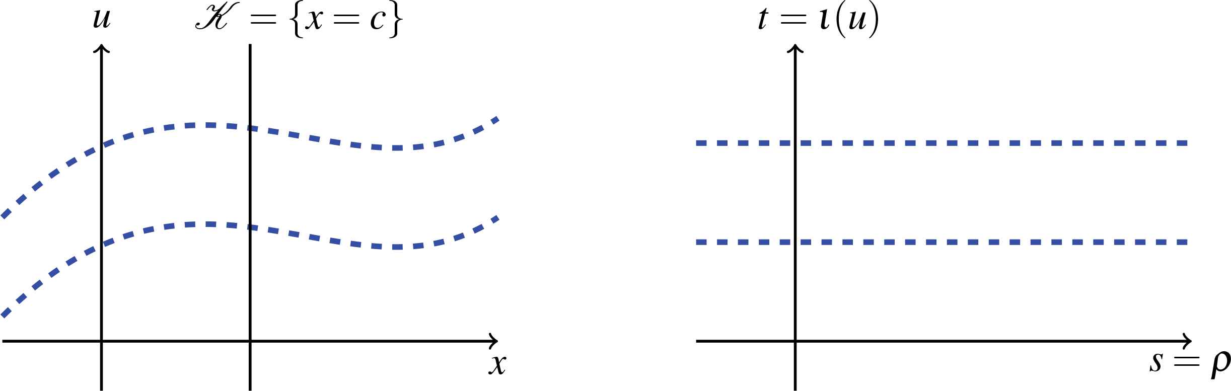
Rectification of the group orbits.

Without relying on the coordinate expressions of t and s, it is possible to compute the derivatives st, stt,…, symbolically. First, we have that

ds=dρ=v=F(t)ϖ, (5.7)
where v = ρ*(μ) is the moving frame pull-back of the Maurer-Cartan form μ. As outlined in the previous section, the function F(t) can be found symbolically using the recurrence relation for the phantom invariant ı(x) = c. In fact, F(t)=1ξ(c,t). Also, the differential dt = dI, is computed symbolically using the recurrence relation for the normalized invariant I = ı(u):
dt=dI=I1ϖ+φ(c,t)v=(I1+φ(c,t)F(t))ϖ,(5.8)
where I1 = ı(ux). Combining (5.7) and (5.8), we have that
st=dsdt=vdt=F(t)I1+φ(c,t)F(t)=1φ(c,t)I1ξ(c,t)=1Q(c,t,I1)=F1(t,I1),
where Q(x, u, ux) = φξ ux is the characteristic of the vector field (5.2). Next, using the recurrence relation for I1 = ı(ux), which is of the form
dI1=(I2+K(t,I1))ϖ,
it is then possible to compute stt symbolically:
stt=dstdt=1dt(F1tdt+F1I1dI1)=F2(t,I1,I2).
Similarly, the recurrence relations for the higher order normalized invariants lead to the symbolic expressions
st=F(t,I1,,I),1.(5.9)
Inverting (5.9), the normalized invariants I can be expressed in terms of t and st, ċ, st:
I=t,I=(t,s(1,)),1,
where s(1,) = (st, ċ, stℓ) collects the derivatives of s with respect to t of order 1 ≤ k. Since the differential equation (5.1) is Gε-invariant, we invariantize the equation to obtain
0=Δ(x,u(n))=ı[Δ(x,u(n))]=Δ(c,I(n))=Δ(c,t,1(t,s(1,1)),,n(t,s(1,n)))=Δ˜(t,s(1,n)).
We observe that the resulting equation Δ˜(t,s(1,n))=0 is independent of s. This was to be expected as in the canonical variables (t, s) the differential equation is invariant under the group of translations (5.6). Introducing the new dependent variable w = st, the order of the original differential equation (5.1) is reduced by one:
Δ˜(t,w(n1))=0.(5.10)

Assuming (5.10) can be solved, we now explain how to recover the solution to the original equation (5.1) without relying on the coordinate expressions of the canonical variables (t, s) (or w = st). We refer to this procedure as the reconstruction step. Let w = w(t) be the general solution to (5.10). Since st = w(t), it follows that

s(t)=w(t)dt.
Next, by definition of the right moving frame, ρ(x,u)=(c,t)K. Inverting the last equality, it follows that
(x,u)=ρ¯(c,t),(5.11)
where ρ¯=ρ1 is the corresponding left moving frame. Since s = ρ and group inversion is given by the additive inverse, equation (5.11) is equivalent to
(x,u)=(s(t))(c,t),(5.12)
where the right-hand side of (5.12) is obtained by acting on the point (c,t)K with the group element −s(t) ∈ G. The latter provides a parametric solution (x(t), u(t)) to the original differential equation (5.1). Inverting the relation x = x(t), to express t as a function of x, we obtain the solution u(t(x)) to the original differential equation (5.1).

Before considering an example, let us summarize the steps involved in the symbolic implementation of the symmetry reduction process introduced above. Starting with the ordinary differential equation (5.1):

  • Compute a basis of infinitesimal symmetry generators following standard procedures, [3, 58,10,1517,27,3537]. Choose one infinitesimal symmetry generator v with respect to which the equation is to be reduced.

  • Let g=span{v} and compute the recurrence relations (4.15) for the lifted invariants of order ≤ n−1

  • Introduce the cross-section (5.4) and let ρ be the corresponding right moving frame. Note, it is not necessary to compute ρ! We only need to know that it exists.

  • Compute the recurrence relations for the normalized invariants I(n)=ı(u(n)) as outlined in Section 4.1

  • Introduce the canonical variables t = ı(u), s = ρ. Invariantizing the differential equation (5.1) and using the recurrence relations for the normalized invariants I(n), rewrite the equation in terms of t, w=dsdt,wt,,wtn1.

  • Solve the reduced equation Δ˜(t,w(n1))=0 to obtain w(t). The solution to the original equation is, in parametric form,

    (x,u)=(s(t))(c,t),
    where s(t)=w(t)dt and the group product is obtained by exponentiating the infinitesimal symmetry generator v.

Example 5.1.

To illustrate the above constructions, consider the first order ordinary differential equation

2x4uux+4x3u2+2x=0.(5.13)
This equation is invariant under the infinitesimal symmetry generator
v=xxuu.
The corresponding group action is
X=eεx,U=eεu,ε,(5.14)
and the order zero lifted recurrence relations are
dX=ω+Xμ,dU=UXωUμ.(5.15)
Choosing the cross-section K={x=1}, the normalized recurrence relations are
0=ϖ+v,dI=I1ϖIv,
where v=ρ*(μ),ϖ=ϱ*(ω). The recurrence relation for the phantom invariant gives v=ϖ. Substituting v into the second equation yields the recurrence relation
dI=(I1+I)ϖ.(5.16)
Invariantizing the differential equation (5.13) we get
2II1+4I2+2=0 so that I1=2I2+1I.
Substituting the latter equality into the recurrence relation (5.16), we obtain
dI=I2+1Iϖ.
Introducing the canonical variables
t=ı(u)=I,s=ρ,
we conclude that
dsdt=vdI=ϖI2+1Iϖ=tt2+1.(5.17)
Setting w = st, equation (5.17) reduces to the algebraic equation
w=tt2+1.
It follows that
s(t)=w(t)dt=12ln(1+t2)+C,
where C is an arbitrary constant of integration. Recalling the group action (5.14), a parametric solution to the original differential equation (5.13) is obtained by acting on the point (1,t)𝒦 by the left moving frame ρ¯=s(t):
x(t)=s(t)1=es(t)=K1+t2,u(t)=s(t)t=es(t)t=t1+t2K,
where K = eC. Solving the first equation for t, and substituting the result into u(t) yields the solution
u(x)=K2x2x2.

5.2. Solvable symmetry group

To extend our symbolic implementation of the symmetry reduction algorithm to solvable symmetry groups, we use the inductive/recursive moving frame constructions outlined in Section 4.2. Our starting point is an nth order ordinary differential equation Δ(x, u(n)) = 0 invariant under the prolonged action of an r-dimensional solvable Lie group G with (3.5) as its chain of normal subgroups. Based on this chain of normal subgroups, we introduce the th lifted subbundle (n)=J(n)×G() and the inclusion map i:(n)G(n) induced by the containment G()G. At the infinitesimal level, let g be the corresponding r-dimensional solvable Lie algebra spanned by the infinitesimal generators v1,…,vr such that (3.7) holds. Dually, let μ1,,μrg* be a basis of Maurer-Cartan forms. Finally, for ∈ {1, . . . , r}, let Gɛ denote the one-parameter Lie group whose local group action on J(0) is induced by the flow of v:

gε(x,u)=exp[εv](x,u),gεGε.

Prior to the implementation of the symmetry reduction algorithm, we first compute the recurrence relations (4.15) for the G-lifted differential invariants of order ≤ n − 1:

d[λG(x)]=ω+=1rλG(ξ)μ,d[λG(uk)]=λG(uk+1)ω+=1rλG(φk)μ,0kn1.(5.18)
Starting the symmetry reduction process, we first implement the procedure outlined in Section 5.1 for the prolonged action of the 1-parameter group Gɛ1 = G(1) on the nth order jet bundle J0(n)=J(n). As in Section 5.1, assume, for simplicity, that x is not an invariant of the Gɛ1-action and consider the cross-section
K1={x=c1}J0(n).
Let ρ1:J0(n)Gε1 be the corresponding right moving frame and let ı1 be the induced invariantization map. We introduce the notation
I;1(n)=ı1(u(n)),ϖ1=ı1(dx),v11=ρ1*(μ1),
to denote the Gɛ1 -normalized differential invariants, the Gɛ1 -invariant horizontal form, and the Gɛ1 - normalized Maurer-Cartan form. To obtain the symbolic expression for v11, first pull-back the lifted recurrence relations (5.18) by the inclusion map i1:1(n)G(n) to obtain the Gɛ1 -lifted recurrence relations
dX=ω1+ξ1(X,U)μ1,dUk=Uk+1ω1+φ1k(X,U(k))μ1,0kn1,(5.19)
where X=λGε1(x),U(k)=λGε1(u(k)) are the Gɛ1-lifted invariants, and ω1=λGε1(dx) is the Gɛ1- lifted horizontal form. Recall that in order to simplify the notation, we purposely omit writing the pull-back map i1*. Also, note that, symbolically, the equations (5.19) are obtained by setting μ2 = ⋯ = μr = 0 in (5.18) and substituting λG(x)X,λG(uk)Uk, and ωω1. Taking the pull-back of (5.19) by the right moving frame section ϱ1:J0(n)1(n), we obtain the recurrence relations for the Gɛ1-normalized differential invariants. The recurrence relation for the phantom invariant ı1(x) = c1 implies that
v11=H1(I;1)ϖ1=ϖ1ξ1(c1,I;1).(5.20)

The recurrence relations for the Gɛ1-normalized differential invariants are then obtained by substituting (5.20) into the remaining recurrence relations, giving

dIk;1=Fk;1(I;1(k+1))ϖ1=(Ik+1;1φ1k(c1,I;1(k))ξ1(c1,I;1))ϖ1,k=0,,n1.
As in the previous section, we introduce the canonical variables
t1=I;1=ı1(u),s1=ρ1,
and let
w1=ds1dt1=v11dI;1=H1(I;1)F;1(I;1(1))=1φ1(c1,I;1)ξ1(c1,I;1)I1;1=1Q1(c,I;1,I1;1),
where Q1(x, u, ux) is the characteristic of the vector field v1. In the variables (t1, w1), the order of the original differential equation (5.1) is reduced by one
Δ(x,u(n))=Δ˜1(t1,w1(n1))=0,
and this completes the first iteration of the symmetry reduction algorithm.

Before proceeding to the second iteration, we recall from Section 5.1 that the normalized invariants I;1(n) can be expressed in terms of (t1,w1(n1)):

I;1=t1,Ik;1=Ik(t1,w1(k1)),1kn1.(5.21)
Therefore, the variables (t1,w1(n1)) provide a local system of coordinates for the cross-section K1,
K1={(c1,t1,w1(n1))}J1(n1)={(t1,w1(n1))},
which is isomorphic to the (n−1)th order jet space J1(n1)={(t1,w1(n1))}.

For the second iteration of the symmetry reduction algorithm, we consider the induced action of the one-parameter group Gɛ2G(2) / G(1) on J1(n1). To obtain the Gɛ2-lifted recurrence relations, we implement the inductive/recursive moving frame constructions introduced in Section 4.2 with G = G(2) and N = G(1). First, we pull-back the lifted recurrence relations (5.18) by the inclusion map i2:2(n)G(n) to obtain the lifted recurrence relations of the G(2)-prolonged action on J(n). Introducing the G(2) lift map λ(2)=λG(2), we have

d[λ(2)(x)]=ω2+λ(2)[ξ1(x,u)]μ1+λ(2)[ξ2(x,u)]μ2,d[λ(2)(uk)]=λ(2)(uk+1)ω2+λ(2)[φ1k(x,u(k))]μ1+λ(2)[φ2k(x,u(k))]μ2,0kn1, (5.22)
where ω2=λ(2)(dx). In the lifted recurrence relations (5.22), we make the substitution λ(2)(x,u(n))=λ(2)(c1,I;1(n)), corresponding to equality (4.22) in the general framework of Section 4.2. This yields the recurrence relations
d[λ(2)(c1)]=ω2+λ(2)[ξ1(c1,I;1)]μ1+λ(2)[ξ2(c1,I;1)]μ2,d[λ(2)(Ik;1)]=λ(2)(Ik+1;1)ω2+λ(2)[φ1k(c1,I1(k))]μ1+λ(2)[φ2k(c1,I;1(k))]μ2, (5.23)
where 0 ≤ kn − 1. Introducing the partial normalization
λ(2)(c1)=c1,
let ρ^G(1):J(n)×Gε2G(2) be the corresponding partial moving frame. Pulling-back the recurrence relations (5.23) by ϱ^G(1)=(id,ρ^G(1)):J(n)×Gε2J(n)×G(2),the first equation becomes
0=ω^2+ξ1(c1,I^;1)μ^1+ξ2(c1,I^;1)μ^2,
where
I^;1=λGε2(I;1)=gε2I;1,gε2Gε2,
ω^2=ϱ^G(1)*(ω2),, and μ^=ρ^G(1)*(μ),=1,2., = 1,2. Solving for μ^1 and substituting the result into the remaining equations of (5.23) gives the lifted recurrence relations for the Lie group Gɛ2 acting on the Gɛ1-normalized invariants of order ≤ n − 1 :
d(I^k;1)=I^k+1;1ω^2+ψ1k(c1,I^;1(k))μ^2,0kn1.(5.24)
The change of variables (5.21), implies that
I^;1=T1,I^k;1=k(T1,W1(k1)),(5.25)
where
T1=λGε2(t1)=gε2t1 and W1(k1)=λGε2(w1(k1))=gε2w1(k1).
Substituting (5.25) into (5.24), we obtain the lifted recurrence relations of the Gɛ2 action on the jet space J1(n1)={(t1,w1(n1))}:
dT1=T(T1,W1)ω^2+ξ(T1,W1)μ^2,dW1;T1k=Wk(T1,W1(k+1))ω^2+φk(T1,W1(k))μ^2,k=0,,n1. (5.26)

Taking the inverse lift λGε21 of the coefficients ξ(T1, W1), φ(T1, W1) multiplying μ^2 in (5.26) we obtain the components of the prolonged vector field v2(1) restricted to J1(0):

v^2=v2(1)|(t1,w1)=ξ(t1,w1)t1+φ(t1,w1)w1.(5.27)
Exponentiating the infinitesimal generator (5.27) gives explicit expressions for the Gɛ2-action on (t1, w1).

With (5.26) in hand, we now implement the second iteration of the symmetry reduction procedure. Again, for simplicity, assume that t1 is not an invariant of the Gɛ2-action, and let K2={t1=c2}J1(n1)be a local cross-section. Let ρ2:J1(n1)Gε2 be the corresponding right moving frame, and ı2 the induced invariantization map. We also introduce the notation

I:2(n1)=ı2(w1(k1)) and ϖ2=ϱ2*(ω^2).
Making the normalization T1 = c2 in (5.26) and solving for the normalized Maurer-Cartan form v22=ϱ2*(μ^2) we obtain
v22=H2(I;2)ϖ2.
Substituting the result into the remaining formulas yields the recurrence relations
dIk;2=Fk;2(I:2(k+1))ϖ2,k=1,,n2.

A new set of canonical variables is introduced by setting

t2=I;2=l2(w1) and s2=ρ2.
Also, let
w2=ds2dt2=v22dI;2=H2(I;2)F;2(I;2(1)).
In the new coordinates (t2, w2), the order of the original differential equation (5.1) is now reduced by two:
Δ˜2(t2,w2(n2))=0.
Also, the jet variables (t2,w2(n2)) can be used to parametrize the cross-section
K2={(c2,t2,w2(n2))}J2(n2)={(t2,w2(n2))}.

The symmetry reduction procedure continues by considering the action of Gɛ3 on the submanifold jet bundle J2(n2)={(t2,w2(n2))} and so on. At the th iteration, the lifted recurrence relations of the Gɛ-prolonged action on the jet space J1(n+1)={(t1,w1(n+1))} is obtained by considering the G()-lifted recurrence relations followed by the normalization of the Maurer-Cartan forms μ1, . . . , μ−1. The latter is achieved by pulling back the G()-lifted recurrence relations with respect to the partial moving frame that keeps the partial cross-section

K={x=c1,t1=c2,,t2=c1}
invariant. Assuming that t−1 is not an invariant of the Gɛ-action, we introduce the cross-section K={t1=c} and let ρ:J1(n+1)Gε be the corresponding right moving frame. The order of the differential equation Δ˜1(t1,w1(n+1))=0 is reduced by one by introducing the canonical variables
t=ı(w1),s=ρ,(5.28)
and rewriting the equation in terms of the variables t,w=dsdtt, and the derivatives of w with respect to t.

At the end of the symmetry reduction algorithm, the fully reduced equation is the order nr differential equation

Δ˜r(tr,wr(nr))=0.(5.29)

Let wr(tr) be the solution to the fully reduced equation (5.29). We now reconstruct the solution to the original differential equation (5.1). By definition wr=dsrdtr, so that

sr(tr)=wrdtr.
Next, since ur(tr−1, wr−1) = ρr ⋅(tr−1, wr−1) = (cr, tr) and ρr = sr, it follows that
tr1=tr1(tr)=ρr1cr=(sr)cr,(5.30a)
γ˙γ˙=qφγ˙.(5.30b)
where the product is given by the Gεr-action on (tr−1, wr−1). Inverting (5.30a), we obtain tr = tr(tr−1). Substituting the result in (5.30b), yields the function wr−1(tr(tr−1)). Repeating the procedure, since wr1=dsr1dtr1 we have
sr1(tr1)=wr1dtr1
and
tr2=(sr1)cr1,wr2=(sr1)tr1,
where the product is now given by the Gɛr−1-action on (tr − 2, wr − 2). Continuing in this fashion, at the last iteration we have
s1=w1dt1
and
x=x(t1)=(s1)c1,u=u(t1)=(s1)t1,
where the product is given by the Gɛ1-action on (x, u). Inverting the relation x = x(t1), to obtain t1 = t1(x), the solution to the original differential equation (5.1) is u(t1(x)).

Before considering two examples, let us summarize the above considerations into a list of executable steps. Our starting point is an nth order ordinary differential equation Δ(x, u(n)) = 0.

  • Compute a basis of infinitesimal symmetry generators using standard techniques, [3,58, 10,1517,27,3537].

  • Find a sufficiently large solvable Lie subalgebra g of dimension r, and let G be the corresponding symmetry group action. Note that we do not have to compute the group action to implement the algorithm. Compute the chain of normal Lie subalgebras (3.6), and consider a canonical basis {v1,…,vr} such that (3.7) holds.

  • Compute the recurrence relations (4.15) for the G-lifted invariants of order ≤ n − 1.

  • Reduce the order of the differential equation Δ(x, u(n)) = 0 iteratively. For 1 ≤ r, the th iteration consists of reducing the differential equationf Δ(t1,w1(n+1))=0. with respect to the one-parameter symmetry group GɛG() / G(− 1) To this end,

    • -Implement the inductive/recursive moving frame constructions with N = G(− 1) and G = G() to obtain the lifted recurrence relations of the Gɛ action on J1(n+1)={(t1,w1(n+1))}. Recall that the G()-lifted recurrence relations are obtained symbolically by setting μ+1 = ċ = μr = 0 in the G-lifted recurrence relations.

    • -Choose a cross-section K={t1=c}J1(n+1) and let ρ be the corresponding right moving frame.

    • -Introduce the canonical variables t, s defined in (5.28), and compute w=dsdtp,dwdtp, and its higher derivatives up to order n +1 symbolically using the recurrence relations for the Gɛ-normalized invariants.

    • -Invariantize Δ˜1(t1,w1(n+1))=0 using the moving frame ρ Writing the result in terms of (t,w(n)) yields the reduced equation

      Δ˜(t,w(n))=0.

  • Let wr(tr) be the solution to the fully reduced equation Δ˜r(tr,wr(nr))=0. The solution to the original differential equation is obtained by implementing the reconstruction process. For 1 ≤ r, the th step consists of:

    • -Evaluating sr+1=wr+1dtr+1.

    • -Computing

      tr(tr+1)=(sr+1)cr+1,wr(tr+1)=(sr+1)tr+1,
      using the Gɛr+1-action on (tr, wr). This action is obtained symbolically from the Gɛr+1-lifted recurrence relations computed in the (r + 1)th reduction step as follows. From the lifted recurrence relations
      dTr=+ξ(Tr,Wr)μ^r+1,dWr=+φ(Tr,Wr)μ^r+1.
      extract the coefficients ξ(Tr,Wr) and φ(Tr,Wr). Their inverse lift yields the coefficients of the vector field
      v^εr+1=ξ(tr,wr)tr+φ(tr,wr)wt.
      Exponentiating v^εr+1 gives the formulas for the Gɛr+1-action on (tr, wr).

    • -Inverting tr = tr(tr+1), and substituting tr+1 = tr+1 (tr) into wr(tr+1), yields wr(tr+1(tr)).

  • The output of the reconstruction process is the solution to the original differential equation Δ(x, u(n)) = 0.

Example 5.2.

We now revisit Example 3.1 using the moving frame machinery. We emphasize the fact that, this time around, computations are performed symbolically without relying on the coordinate expressions of the canonical variables and the differential invariants.

Since the differential equation is of order two, we consider the lifted recurrence relations (4.17) of the full symmetry group (4.2) up to order one. According to the solvable structure of the symmetry group, we first implement the symmetry reduction process using the one-parameter group Gɛ1. The recurrence relations for the Gɛ1-lifted invariants were obtained in (4.32). Choosing the crosssection (4.27), let ρ1 be the corresponding right moving frame and let l1 be the induced invariantization map. Using the same notation as in (4.29), the recurrence relations for the Gɛ1-normalized invariants are given in (4.35).

We now introduce the canonical variables

t=ı1(x)=H,s=ρ1.
Using (4.34) and the recurrence relations (4.35), we have that
st=dsdt=v1dH=I1H,
and
stt=dstdt=1ϖ1d(I1H)=1ϖ1(dI1H+I1H2dH)=I2H+2I1H2.
Therefore,
I1=tst and I2=tstt2st.
Introducing the variable w = st,
I1=tw and I2=twt2w.(5.31)
Invariantizing the differential equation (3.8), we obtain
H2I2=F(HI1),
which when expressed in the variables (t, w(1)), yields the first order differential equation
t3wt+2t2w=F(t2w).(5.32)

Now, let Gɛ2 act on J1(1)={(t,w(1))}. To obtain the corresponding Gɛ2-lifted recurrence relations, recall that the recurrence relations for the Gɛ2-lift of the Gɛ1-normalized invariants (H, I1, I2, …) were obtained in (4.36). Using (5.31), we have that

H^=gε2H=gε2t=T,I^1=gε2I1=gε2(tw)=TW,I^2=gε2I2=gε2(twt2w)=TWT2W. (5.33)
Substituting (5.33) into the first two equations of (4.36), we obtain
dT=ω^+Tμ^2,dW=WTω^2Wμ^2.(5.34)
Assuming T > 0, a cross-section to the Gɛ2-action is given by
K2={t=1},
which is equivalent to making the normalization T = 1. Let ρ2 be the induced right moving frame and ı2 the corresponding invariantization map. Also, let
J=ı2(w),J1=ı2(wt),v2=ϱ2*(μ^2),σ2=ϱ2*(ω^).
Then, the normalized recurrence relations are
0=ϖ2+v2,J=J1ϖ22Jv2.
The first equation gives
v2=ϖ2,
which when substituted into the second equation yields
dJ=(J1+2J)ϖ2.(5.35)
Invariantizing (5.32) we find that
J1=(2J+F(J)).(5.36)
Substituting (5.36) into (5.35) yields
dJ=F(J)ϖ2.
Introducing the canonical variables
y=J,z=ρ2,
where z = z(y), we have that
zy=dzdy=v2dJ=1F(y).

As in Example 3.1, assume F(−y) = y2. Then

zy=1y2 so that z=1y+lnC.(5.37)

Given (5.37), we now recover the solution to the original differential equation (3.15). Taking the inverse lift of the coefficients multiplying μ^2 in (5.34), i.e. λε21(T)=t and λε21(2W)=2w, we obtain the infinitesimal generator

v^2=tt2ww.
This vector field induces the one-parameter group action
T=eε2t,W=e2ε2w.
Since
1=ı2(t)=eρ2t,y=J=t2(w)=e2ρ2w,
and ρ2 = z, it follows that
t=ez=1Ce1/y and w=e2zy=C2ye2/y,
From the first equation y=1ln(Ct), which when substituted into the expression for w yields
w(t)=1t2ln(Ct).
Since w = st,
s(t)=w(t)dt=CE1(ln(Ct))K.
Setting ε2 = 0 in (4.2) we see that Gɛ1 acts on (x, u) by Galilean boosts:
X=x,U=u+ε1x.
Recalling that
t=H=ı1(x)=x and 0=ı1(u)=u+ρ1x=u+sx,
we conclude that the general solution to the original differential equation (3.15) is
u=xs(x)=CxE1(ln(Cx))+Kx.
As expected, we recover the same solution as in Example 3.1, with the important distinction that the coordinate expressions for the canonical variables and the differential invariants were not used in the derivation of the solution.

Remark 5.1.

The choice of canonical variables is not unique. For example, in Example 3.1 the general solution to the system of differential equations (3.10) is

t=f(x),s=ux+g(x),(5.38)
where fx ≠ 0 and g is an arbitrary smooth function. The canonical variables introduced in (3.11) correspond to the simplest possible solution.

This freedom in the choice of the canonical variables also appears in the moving frame approach. First, the choice of the cross-section (4.27) is not unique. If it were replaced by

K1={u=xg(x)},
then the solution to the normalization equation − x g(x) = U = u + ε1x would give
s=ε1=uxg(x),
recovering, up to a sign, the second canonical variable in (5.38). Also, since the function of an invariant is an invariant function, the definition of the canonical variable
t=ı1(x)=x
can be extend to
t=f(l1(x))=f(x),
where fx ≠ 0. In doing so we recover the first canonical variable in (5.38).

From a purely symbolic and computational standpoint, the symmetry reduction algorithm can be executed using solely the lifted recurrence relations of the the whole symmetry group G. Reviewing the general procedure outlined above, we notice that in the first iteration of the symmetry reduction algorithm, all computations can be carried out using the lifted recurrence relations for G provided the equalities are defined modulo the Maurer-Cartan forms μ2,…,μr. Similarly, in the second iteration, all computations hold modulo the Maurer-Cartan forms μ3,…,μr. In general, at the th iteration, the first − 1 Maurer-Cartan forms μ1,…,μ − 1 will have been (partially) normalized and the symmetry reduction computations can be performed using the recurrence relations of the whole symmetry group provided the equalities are defined modulo the (partially normalized) Maurer-Cartan forms μ^+1,,μ^r. By working with the recurrence relations of the whole symmetry, the computations and the implementation of the symmetry reduction algorithm becomes more straightforward. This is illustrated in the following example.

Example 5.3.

Consider the second order ordinary differential equation

uxx=uxu21xu.(5.39)
Equation (5.39) admits a two-dimensional symmetry group G with infinitesimal generators
v1=x2x+xuu,v2=xxu2u,
and first prolongation
v1(1)=x2x+xuu+(uxux)ux,v2(1)=xxu2u+ux2ux.
The lifted recurrence relations of the whole symmetry group G are, up to order 1,
dX=ω+X2μ1Xμ2,dU=UXω+XUμ1U2μ2,dUX=UXXω+(UXUX)μ1+UX2μ2. (5.40)
Since
[v1,v2]=v1,
we first reduce equation (5.39) using the 1-parameter group induced by the infinitesimal generator v1. Let ρ1:J(2)Gε1(2) be the moving frame obtained by normalizing X = 1 and let ı1 be the induced invariantization map. Working with the 2-parameter group G, let ρ^1 be the partial moving frame obtained by normalizing X = 1. Also, let
I^k=ρ^1Ik,ω^=ϱ^1*(λG(ϖ1)),μ^1=ρ^1*(μ1),μ^2=ρ^1*(μ2),
where Ik = ı1 (uk) and ϖ1=t1(dx). Pulling back the lifted recurrence relations (5.40) by the section ϱ^1 induced by the partial moving frame ρ^1, we obtain
0=ω^+μ^1μ^2,dI^=I^1ω^+I^μ^1I^2μ^2,dI^1=I^2ω^+(I^I^1)μ^1+I^12μ^2.
Since we are performing symmetry reduction with respect to v1, we use the first equation to solve for μ^1:
μ^1=ω^+μ^2.(5.41)
Substituting the result into the remaining equations yields
dI^=(I^1I^)ω^+I^2μ^2,dI^1=(I^2+I^1I^)ω^+(I^I^12)μ^2.(5.42)
Modulo μ^2, we obtain
dI^(I^1I^)ω^,dI^1(I^2+I^1I^)ω^.(5.43)
The recurrence relations for the Gɛ1-normalized invariants I = ı1 (u), I1 = ı1 (ux) are symbolically obtained by dropping the hat notation over the invariants in (5.43) and substituting ω^σ1=ı1(dx):
dI=(I1I)ϖ1,dI1=(I2+I1I)ϖ1.
Also, modulo μ^2, equation (5.41) becomes μ^1ω^, from which we conclude that v1=ρ1*(μ1)=ϖ1. Introducing the canonical variables t = I, s = ρ1, and setting w = st, we have that
w=st=v1dI1I1I and wt=stt=I2(I1I)3.(5.44)
Invariantizing (5.39) we obtain the reduced differential equation
wt=w2t2.(5.45)

We now reduce (5.45) using the 1-parameter group Gɛ2 induced by the infinitesimal generator v2. From (5.44), we have that

I=t,I1=t1w,I2=wtw3.
Making the substitutions
I^T,I^1T1W,I^2WTW3,
into (5.42), we obtain the order zero Gɛ2-lifted recurrence relations
dT=1Wω^+T2μ^2,dW=WTWω^+W2μ^2.(5.46)
Let ρ2:J1(1)={(t,w,wt)}Gε2 be the moving frame obtained by normalizing T = 1, and let ı2 be the corresponding invariantization map. Introducing the notation
J=ı2(w),J1=ı2(wt),ϖ2=ϱ2*(ω^),v2=ϱ2*(μ^2),
and pulling back (5.46) by the moving frame section ϱ2 we obtain
0=1Jϖ2+12v2,dJ=J1Jϖ2+J2v2.
The first equation implies that
v2=2Jϖ2.(5.47)
Substituting (5.47) into the second equation yields the recurrence relation
dJ=(1J1J)ϖ2.(5.48)
Invariantizing (5.45) we obtain the syzygy J1 = J2, which when substituted in (5.48) yields
dJ=(1J)ϖ2.
Introducing the canonical variables y = J and z = ρ2, with z = z(y), we have that
zy=dzdy=v2dJ=2y(1y).
Integrating the latter equation gives
z(y)=ln(Cy1y)2.

We now recover the solution to the original differential equation (5.39) by implementing the reconstruction process. Un-lifting the coefficients multiplying μ^2 in (5.46), we conclude that

v^2=v2(1)|(t,w)=t2t+w2w.
Therefore, Gɛ2 acts on (t, w) by dilation:
T=eε22 t,W=e ε22 w.
Since l2(t, w) = ρ2 ⋅(t, w) = (1, y), we have
t=eρ221=ez2=1yCy so that y=1Ct+1,
and
w=eρ22y=ez2y=1yC=tCt+1.
Hence,
st=w=tCt+1 and s(t)=tC1C2ln(Ct+1)+K.
Finally, since the action of Gɛ1 on (x, u) is given by
X=x1ε1x ,U=u1ε1x ,
acting on ı1 (x,u)=(1,t) by the left moving frame ρ¯1=s(t) yields the parametric solution
x=11+s=C2Ct+Bln(Ct+1),u=t1+s=C2tCt+Bln(Ct+1),
to the differential equation (5.39).

Acknowledgment

The author would like to thank the referees for their comments and suggestions, which helped improve the exposition of paper.

Footnotes

a

Given an infinitesimal generator, the corresponding (local) one-parameter group action is obtained by exponentiating the vector field, see (2.4).

b

The subalgebra g(1) is also called an ideal of g(), [15].

c

Any two-dimensional Lie algebra is solvable.

d

A differential one-form Ω on J(n) is contact-invariant if and only if, for every gG, g * Ω = Ω + θg for some contact form θg

e

In its most general formulation, the universal recurrence formula is stated for a differential form defined on J(∞).

f

When = 1, we let Δ0(t0,w0(n))=Δ(x,u(n))=0.

References

[2]I.M. Anderson, The Variational Bicomplex, Technical Report, Utah State University, 2000.
[3]D.J. Arrigo, Symmetry Analysis of Differential Equations: An Introduction, John Wiley & Sons, New Jersey, 2015.
[4]J. Benson, Integrable equations and recursion operators in planar Klein geometries, Lob. J. Math., Vol. 36, 2015, pp. 234-244.
[5]G.W. Bluman and S.C. Anco, Symmetry and Integration Methods for Differential Equations, Springer–Verlag, New York, 2002. Applied Mathematical Sciences, Vol. 154
[6]G.W. Bluman, A. Cheviakov, and S.C. Anco, Applications of Symmetry Methods to Partial Differential Equations, Springer–Verlag, New York, 2010. Applied Mathematical Sciences, Vol. 168
[7]L.A. Bordag, Geometrical Properties of Differential Equations: Applications of the Lie Group Analysis in Financial Mathematics, World Scientific Publishing Company, New Jersey, 2015.
[8]B.J. Cantwell, Introduction to Symmetry Analysis, Cambridge Text in Applied Mathematics, Cambridge University Press, Cambridge, 2002.
[10]L. Dresner, Applications of Lie’s Theory of Ordinary and Partial Differential Equations, Institute of Physics Publishing, Philadelphia, 1999.
[15]P. Hydon, Symmetry Methods for Differential Equations: A Beginner’s Guide, Cambridge Text in Applied Mathematics, Cambridge University Press, Cambridge, 2000.
[16]N.H. Ibragimov, Selected Works, Vol. 1,2, and 3, ALGA Publications, Sweden, 2006.
[17]N.H. Ibragimov and R.N. Ibragimov, Applications of Lie Group Analysis in Geophysical Fluid Dynamics, World Scientific, China, 2011. CNC Series on Complexity, Nonlinearity and Chaos Vol. 2
[22]E.L. Mansfield, A Practical Guide to the Invariant Calculus, Cambridge Monographs on Applied and Computational Mathematics, Cambridge University Press, Cambridge, 2010.
[26]K. Oldham, J. Myland, and J. Spanier, The exponential integrals Ei(x) and Ein(x), An Atlas of Functions, 2nd edn., Springer, New York, 2008, pp. 375-384.
[27]P.J. Olver, Applications of Lie Groups to Differential Equations, 2nd edn., Springer–Verlag, New York, 1993. Graduate Text in Mathematics, Vol. 107
[31]P.J. Olver, Modern developments in the theory and applications of moving frames, London Math. Soc. Impact150 Stories, Vol. 1, 2015, pp. 14-50.
[34]P.J. Olver and F. Valiquette. Recursive moving frames for Lie pseudo-groups, Preprint, University of Minnesota, 2016
[35]L.V. Ovsiannikov, Group Analysis of Differential Equations, Academic Press, New York, 1982.
[36]L.V. Poluyanov, A. Aguilar, and M. González, Group Properties of the Acoustic Differential Equation, Taylor & Francis Inc., Bristol, 1995.
[37]H. Stephani, Differential Equations: Their Solution Using Symmetries, Cambridge University Press, Cambridge, 1989.
[39]R. Thompson and F. Valiquette, Group foliation of differential equations using moving frames, Forum of Mathematics: Sigma, Vol. 3, 2015, pp. 53. e22
[41]F. Valiquette, Solving local equivalence problems with the equivariant moving frame method, SIGMA, Vol. 9, 2013, pp. 43. 023
Journal
Journal of Nonlinear Mathematical Physics
Volume-Issue
25 - 2
Pages
211 - 246
Publication Date
2021/01/06
ISSN (Online)
1776-0852
ISSN (Print)
1402-9251
DOI
10.1080/14029251.2018.1452671How to use a DOI?
Copyright
© 2018 The Authors. Published by Atlantis and Taylor & Francis
Open Access
This is an open access article distributed under the CC BY-NC 4.0 license (http://creativecommons.org/licenses/by-nc/4.0/).

Cite this article

TY  - JOUR
AU  - Francis Valiquette
PY  - 2021
DA  - 2021/01/06
TI  - Symmetry Reduction of Ordinary Differential Equations Using Moving Frames
JO  - Journal of Nonlinear Mathematical Physics
SP  - 211
EP  - 246
VL  - 25
IS  - 2
SN  - 1776-0852
UR  - https://doi.org/10.1080/14029251.2018.1452671
DO  - 10.1080/14029251.2018.1452671
ID  - Valiquette2021
ER  -