Magnetic curves in Sol₃

Zlatko Erjavec; Jun-ichi Inoguchi

doi:10.1080/14029251.2018.1452670

<Previous Article In Issue

Download article (PDF)

Next Article In Issue>

Volume 25, Issue 2, March 2018, Pages 198 - 210

Magnetic curves in Sol₃

Authors

Zlatko Erjavec

Faculty of Organization and Informatics, University of Zagreb, Pavlinska 2, Varaždin, HR-42000, Croatia,zlatko.erjavec@foi.hr

Jun-ichi Inoguchi

Institute of Mathematics, University of Tsukuba, 1-1-1 Tennodai, Tsukuba, 305-8571, Japan,inoguchi@math.tsukuba.ac.jp

Received 5 August 2017, Accepted 7 November 2017, Available Online 6 January 2021.

DOI: 10.1080/14029251.2018.1452670 How to use a DOI?
Keywords: magnetic curves; contact structure; Sol space
Abstract: Magnetic curves with respect to the canonical contact structure of the space Sol₃ are investigated.
Copyright: © 2018 The Authors. Published by Atlantis and Taylor & Francis
Open Access: This is an open access article distributed under the CC BY-NC 4.0 license (http://creativecommons.org/licenses/by-nc/4.0/).

Introduction

In electromagnetic theory, magnetic curves represent the trajectories of charged particles moving in Euclidean 3-space 𝔼³ under a static magnetic field B→. Newton's second law of motions under the Lorentz force derived from a static magnetic field implies the law of Lorentz force. More precisely, a particle of mass m and charge q on position r→(t) in a static magnetic field B→ moves with the velocity v→(t) satisfying the Lorentz equation

mdv→dt(t)=qv→(t)×B→r→(t).

As is well known, in 𝔼³ the motion of the particle is described by a circular helix around B→. Particularly, magnetic trajectories of the particle can be circles (and hence periodic curves).

The notion of a static magnetic field can be generalized to arbitrary Riemannian manifolds (see [2,25]). Let (M, g, F) be a Riemannian manifold with a closed 2-form F. Then F is referred to as a magnetic field on M. A curve γ(t) is called a magnetic curve if it satisfies the Lorentz equation:

∇γ˙γ˙=qφγ˙.

Here q is a constant (called the charge), ∇ is the Levi-Civita connection and φ is an endomorphism field metrically related to the magnetic field F via g. Hence geodesics in Riemannian manifolds are mathematical models of motions of particles without the Lorentz force or charge 0.

On the other hand, according to Thurston, there are eight model spaces in 3-dimensional homogeneous geometries.

space forms: Euclidean 3-space E3, 3-sphere S3, hyperbolic 3-space ℍ3,
product spaces: S2×ℝ,ℍ2×ℝ,
the Heisenberg group Nil₃, the universal covering SL˜2ℝ of SL2ℝ,
the Sol ₃ space.

Among these eight model spaces, S3 Nil₃ SL˜2ℝand Sol₃ admits a contact structure compatible to the metric (see [24]). The compatible contact structure naturally induces a magnetic field F (called a contact magnetic field ) on these four model spaces.

The study of magnetic curves in arbitrary Riemannian manifolds was developed in early 1990’s, even though related works can be found earlier (see [10,25]). The notation used here is very similar to notation used in [7] and [8].

In 2009 Cabrerizo et al. have looked for periodic orbits of the contact magnetic field on the unit 3-sphere S3 in [7]. In addition, Druţă-Romaniuc et al. classified magnetic trajectories in Nil₃ and SL˜2ℝ with respect to a contact magnetic field [8]. Magnetic trajectories on the space Sol₃ with respect to a contact magnetic field are not studied, yet.

The purpose of this paper is to study magnetic trajectories in the model space Sol₃ of solvegeometry with respect to a contact magnetic field.

1. Magnetic curves

Let (M, g) be a Riemannian manifold. We equip a closed 2-form F on M. Thus we get an endomorphism field φ by

g(φX,Y)=F(X,Y).(1.1)

We regard F as a (mathematical model of ) magnetic field (see [2,25]). And the endomorphism field φ is referred to as the Lorentz force derived from F.

Then a magnetic trajectory γ (also called a magnetic curve) is defined as a solution to

∇γ′γ′=qφγ′.(1.2)

Here q is a real constant called the charge of the magnetic trajectory γ(t) under the magnetic field F

It is well-known that magnetic trajectories have constant speed. When a magnetic curve γ(s) is arc length parametrized, it is called a normal magnetic curve.

One can see that the differential equation of magnetic trajectory is a generalization of geodesic equation. In fact if φ = 0, i.e. F = 0 or q = 0, the differential equation coincides with geodesic equation.

On a Riemannian manifold (M, g, F) equipped with an exact magnetic field F = dA, one can consider the variational problem for regular curves γ(t) with respect to the following Landau-Hall functional:

LH(γ)=∫0ℓ12g(γ′(t),γ′(t))dt−q∫0ℓA(γ′(t))dt.

Here q is a real constant

Let p and p′ be distinct points. Denote by C^∞[a, b] the space of smooth curves in M defined on a closed interval [a, b] satisfying the boundary condition

γ(a)=p, γ(b)=p′.

Take a variation γ_ε through γ(. i.e., γ₀(s) = γ(s)) satisfying the boundary condition

γε(a)=p, γε(b)=p′.

Then the first variation formula of the Landau-Hall functional is given by (see e.g. [11]):

ddε|ε=0LH(γε)=−∫0ℓg(∇γ′γ′−qφγ′,V(s))ds,

where V is the variational vector field

V(s)=∂∂ε|ε=0γε(s).

Thus the Euler-Lagrange equation of this variational problem is exactly the magnetic equation (1.2).

Note that the magnetic equation (1.2) makes sense even if F is not exact.

Remark 1.1.

Magnetic curves with respect to non-standard magnetic fields on Euclidean 3-space E3 are used in computer aided geometric design (see [29] and [30]).

2. Contact structures

Let M be a 3-dimensional manifold. A 1-form η is said to be a contact form if it satisfies dη∧η≠0. A 3-dimensional manifold M together with a contact form η is called a contact 3-manifold. Luts and Martinet proved that every compact orientable 3-manifold carries a contact form (see [19,20,27]).

On a contact 3-manifold (M, η), there exists a unique vector filed ξ such that η(ξ) = 1 and lξdη=0. The vector field ξ is called the Reeb vector field of (M, η). In analytical mechanics, ξ is traditionally called the characteristic vector field of (M, η).

Moreover, every contact 3-manifold (M, η) admits an endomorphism field φ and a Riemannian metric g such that (see [3]):

φ2=−I+η⊗ξ, η∘φ=0,φξ=0,

g(φX,φY)=g(X,Y)−η(X)η(Y),X,Y∈X(M),(2.1)

and

dη(X,Y)=g(X,φY),X,Y∈X(M).(2.2)

Here X(M) denotes the Lie algebra of all smooth vector fields on M. The exterior derivative dη of η is defined by

dη(X,Y)=12(Xη(Y)−Yη(X)−η([X,Y])),

for any X,Y∈X(M).

The structure (φ, ξ, η, g) is called an almost contact metric structure associated to the contact form η . The resulting space (M, φ, ξ, η, g) is called a contact metric 3-manifold. Note that the volume element of a contact metric 3-manifold M is −η∧dη/2.

Remark 2.1.

On a contact 3-manifold (M, η) equipped with an arbitrary chosen Riemannian metric g, one can take a magnetic field F = k dη(k is a nonzero constant ) and consider magnetic curves with respect to F and g. It seems to be natural to demand that the metric g satisfies some “compatibility condition” (see e.g. (2.1)) with respect to F. In this paper we restrict our attention to Riemannian metrics satisfying the condition:

g(X,φY)=kdη(X,Y),X,Y∈X(M).

Remark 2.2.

Perrone in [24] classified homogeneous contact metric 3-manifolds. According to [24], among the simply connected model spaces of Thurston geometry, the following spaces admit a homogeneous contact form compatible to the metric:

S3, Nil3, SL˜2ℝ, Sol3.

For more information on contact forms on compact 3-manifolds with universal cover SL˜2ℝ and Sol₃ refer to [22].

3. Invariant contact structure on Sol₃

3.1. Model of the Sol₃ space

In this subsection we recall relevant facts on Sol₃ given in [5, 6, 9,13–8].

The model space Sol₃ of solvegometry in the sense of Thurston (see [26]) is the Cartesian 3-space ℝ3(x,y,z) equipped with a homogeneous Riemannian metric

g=e2zdx2+e−2zdy2+dz2.(3.1)

The Sol₃ space is a Lie group G with respect to the multiplication law:

(x,y,z)*(a,b,c)=(x+e−za,y+ezb,z+c).

The unit element is (0,0, 0) and the inverse element of (x, y, z) is (−e^zx,−e⁻^zy,−z) . The left translated vector fields associated to the orthonormal basis E^1=(1,0,0),E^2=(0,1,0),E^3=(0,0,1) are

e^1=e−z∂∂x, e^2=ez∂∂y, e^3=∂∂z.(3.2)

The space Sol₃ can be realized as the closed subgroup

{(e−z0x0ezy001)∣x,y,z∈ℝ}

of SL3ℝ. The corresponding Lie algebra sol3 is

{(−w0u0wv000)∣u,v,w∈ℝ}.

The orthonormal basis {E^1,E^2,E^3} of sol3 is identified with

E^1=(001000000), E^2=(000001000), E^3=(−100010000).

The dual coframe field ϑ=(θ1,θ2,θ3) of ℰ={e^1,e^2,e^3} is

θ1=ezdx,θ2=e−zdy,θ3=dz.(3.3)

The connection 1-forms {ω_jⁱ} defined by dθi+∑k=13ωji∧θj=0 relative to ϑ are

(ωji)=(00θ100−θ2−θ1θ20).

The curvature 2-forms {Ωji} defined by Ωji=dωji+∑k=13ωki∧ωjk relative to ϑ are

(Ωji)=(0θ1∧θ2−θ1∧θ3−θ1∧θ20−θ2∧θ3θ1∧θ3θ2∧θ30)

In covariant derivative fashion, the Levi-Civita connection ∇ of Sol₃ is described as follows

∇e^1e^1=−e^3,∇e^1e^2=0,∇e^1e^3=e^1,∇e^2e^1=0,∇e^2e^2=e^3,∇e^2e^3=−e^2,∇e^3e^1=0,∇e^3e^2=0,∇e^3e^3=0.(3.4)

The Riemannian curvature R is defined by

R(X,Y)Z=∇X∇YZ−∇Y∇XZ−∇[X,Y]Z,X,Y,Z∈X(M).

The Riemannian curvature R is expressed in components Rkijℓ by

R(e^i,e^j)e^k=∑ℓ=13Rkijℓe^ℓ

is computed as

R2121=1,R3131=−1,R3232=−1.

The Ricci tensor field Ric is defined by

Ric(X,Y)=tr(Z↦R(Z,X)Y).

The components Rij=Ric(e^i,e^j)=∑l=13Ril jl. is given by

R11=0,R22=0,R33=−2

The scalar curvature ρ:=trRic=∑i=13Rii is −2.

3.2. Invariant contact structure on Sol₃

In this subsection, we introduce a left invariant contact structure on Sol₃.

For more about a left invariant contact structures see [4,14,24].

On the solvable Lie group Sol₃, we may take the following left invariant orthonormal frame field:

e1:=12(e^1−e^2),e2:=e^3,e3:=12(e^1+e^2).(3.5)

Here the orthonormal frame field {e^1,e^2,e^3} is defined by (3.2).

We choose ξ: = e₃ and denote by η the metrical dual 1-form of ξ. Namely η is given by

η=12(ezdx+e−zdy).

Then η is a left invariant contact form on Sol₃. Next we define an endomorphism field φ by

φe1=−e2,φe2=e1,φe3=0.(3.6)

Then φ and ξ are also left invariant on Sol₃. Direct calculations show that

dη(X,Y)=12g(φX,Y), X,Y∈X(Sol3).(3.7)

Remark 3.1.

Precisely speaking, to adapt to contact metric geometry, we need to perform the following normalization procedure:

φ↦−φ, ξ↦2ξ,η↦12η,g↦14g.

Then the resulting quintet (Sol₃,−φ, 2ξ, η / 2, g / 4) is a contact metric manifold (in the sense of [3]) as explained in Section 2.

However, in the study of magnetic curves, this normalization is not essential. So we do not use this normalization hereafter (cf. Remark 2.1).

According to (3.4) and (3.5), the Levi-Civita connection ∇ of Sol₃ is rewritten as

∇e1e1=0,∇e1e2=e3,∇e1e3=−e2,∇e2e1=0,∇e2e2=0,∇e2e3=0,∇e3e1=−e2,∇e3e2=e1,∇e3e3=0.(3.8)

The commutation relations are

[e1,e2]=e3, [e2,e3]=−e1, [e3,e1]=0.

Thus {e₁, e₂, e₃} is a unimodular basis of sol3[21].

The sectional curvature K is determined by

K(e1∧e2)=−1, K(e2∧e3)=−1, K(e1∧e3)=1.

4. Magnetic curves in Sol ₃

4.1. Contact magnetic fields

Let M = (M, φ, ξ, η, g) be a contact metric 3-manifold. Then for a constant k, F = kdη is a magnetic field on M. The magnetic field F = kdη is called the contact magnetic field on a contact metric 3-manifold M. Magnetic trajectories with respect to contact magnetic fields are called contact magnetic trajectories.

Contact magnetic trajectories on the 3-sphere are investigated in [7]. Munteanu and Nistor studied periodicity of contact magnetic fields on 3-tori [23].

In the case of Sol₃ equipped with the structure (φ, ξ, η, g) defined in Section 3.2, we take the contact magnetic field F given by (see (3.7)).

F(X,Y)=2dη(X,Y),X,Y∈X(Sol3).(4.1)

Then the corresponding Lorentz force coincides with φ.

The magnetic curve equation on Sol₃ with respect to F = 2dη with charge q is

∇γ′γ′=qφγ′.(4.2)

Note that contact magnetic equation (4.2) is the Euler-Lagrange equation of the Landau-Hall functional

LH(γ)=∫0ℓ12g(γ′(s),γ′(s))ds−2q∫0ℓη(γ′(s))ds.

4.2. Magnetic curve equation

First task is to deduce the magnetic curve equation (4.2) for a regular curve γ(s) = (x(s), y(s), z(s)) in Sol₃. We have

γ′(s)=x′(s)∂∂x+y′(s)∂∂y+z′(s)∂∂z,

and from (3.2) and (3.5) it follows

γ′(s)=x′(s)ez2(e1+e3)−y′(s)e−z2(e1−e3)+z′(s)e2

and hence

γ′(s)=12(ezx′(s)−e−zy′(s))e1+z′(s)e2+12(ezx′(s)+e−zy′(s))e3.(4.3)

Next we compute the covariant derivative ∇γ′γ′.

∇γ′γ′=12(ezx″−e−zy″+2z′(ezx′+e−zy′))e1+(z″+e−2z(y′)2−e2z(x′)2)e2+12(ezx″+e−zy″+2z′(ezx′−e−zy′))e3.

Taking in account relations (4.3) and (3.6) we have

φγ′=z′e1−12(ezx′−e−zy′)e2.

Hence from the magnetic curve equation (4.2) we obtain system of differential equations

ezx″−e−zy″+2z′(ezx′+e−zy′)=2qz′,z″+e−2z(y′)2−e2z(x′)2=−12q(ezx′−e−zy′),ezx″+e−zy″+2z′(ezx′−e−zy′)=0,(4.4)

Remark 4.1.

Notice that the system of differential equations (4.4) for q = 0 coincides with the system of differential equations (4.4) in [6] which determines geodesics in Sol₃(cf. [5,28]).

Without loss of generality, we can restrict our attention to magnetic trajectories under the initial conditions:

x(0)=0, y(0)=0, z(0)=0, x′(0)=a, y′(0)=b, and z′(0)=c,

since Sol₃ is a homogeneous Riemannian space.

After the summing of the first and the third equation of the system (4.4) we obtain

x″+2x′z′=22qe−zz′.(4.5)

Solving this ODE in the first step we get

x′(s)=(a−q2)e−2z(s)+q2e−z(s)(4.6)

and finally

x(s)=(a−q2)∫0se−2z(τ)dτ+q2∫0se−z(τ)dτ.(4.7)

Analogously for y-coordinate, after subtracting the first from the third equation of the system (4.4) we obtain following equation

y″−2y′z′=−22qezz′.(4.8)

Hence

y′(s)=(b−q2)e2z(s)+q2ez(s)(4.9)

and

y(s)=(b−q2)∫0se2z(τ)dτ+q2∫0sez(τ)dτ.(4.10)

Substituting (4.6) and (4.9) in the second equation of the system (4.4) we get

z″+(b−q2)2e2z−(a−q2)2e−2z+q2((b−q2)ez−(a−q2)e−z)=0(4.11)

Now we assume that s is an arc length parameter of γ. If we multiply this equation by 2z′(≠ 0), after integrating and usingz′(0)=c=1−a2−b2, we obtain

(z′)2+[(a−q2)e−z+q2]2+[(b−q2)ez+q2]2=1(4.12)

After separation of variables, the solution of this equation is given by the following elliptic integral

dz±1−[(a−q2)e−z+q2]2−[(b−q2)ez+q2]2=ds(4.13)

Hence, the following theorem is proved.

Theorem 4.1.

The normal magnetic curves of the space Sol₃ with respect to the contact magnetic field F = 2dη with charge q ≠ 0 is given by the following equations:

x(s)=(a−q2)∫0se−2z(τ)e−2z(τ)+q2∫0se−z(τ)dτ,y(s)=(b−q2)∫0se2z(τ)dτ+q2∫0sez(τ)dτ,ds=dz±1−[(a−q2)e−z+q2]2−[(b−q2)ez+q2]2,

where a,b,c∈ℝ and a² + b² + c² = 1

In the sequel we consider particular cases of magnetic curves in Sol₃.

Example 1

First we examine case z′ = 0 . Then (4.12) implies z = 0 and from (4.7) and (4.10) it follows

γ(s)=(as,bs,0)(4.14)

where a,b∈ℝ. It is a (geodesic) line in the plane z = 0.

Example 2

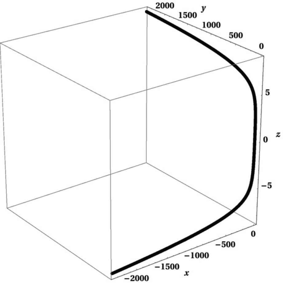
If we assume that a=b=q2, then from (4.12),(4.7) and (4.10) it follows

γ(s)=(−q⋅e−(1−q2⋅s)2(1−q2),q⋅e(1−q2⋅s)2(1−q2),1−q2⋅s).(4.15)

Particularly, for q = 0 we have the z-axis, which is a geodesic line in Sol₃ space.

Figure 1 shows the magnetic curve for a=b=q2, q=12, s ∈ [−10, 10].

Example 3

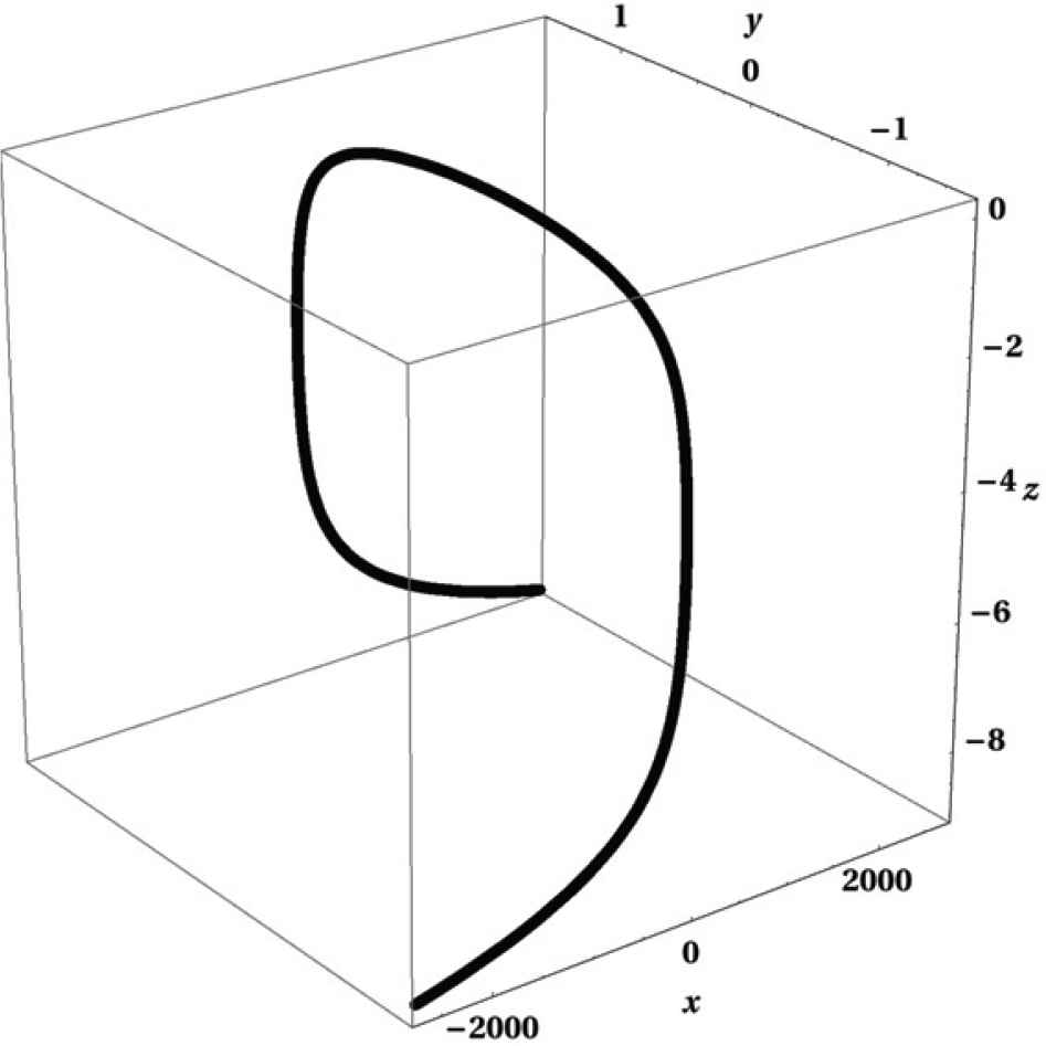
If we assume a=q2, then from (4.11) we have

z″+(b−q2)2e2z+q2(b−q2)ez=0(4.16)

The solution of this equation is

z(s)=−ln[(b−q2)(1+q22coshs+q2)].

Further, from (4.7) and (4.10) it follows

x(s)=q⋅(2b−2q)4(q⋅s+2+q2⋅sinhs),y(s)=2(2b−2q)2+q2⋅sinhs(q+2+q2⋅coshs).

Particularly, for q = 0 we obtain geodesic line in yz-plane.

Figure 2 shows the magnetic curve for b = 1, q=12, s ∈ [−10, 10].

Example 4

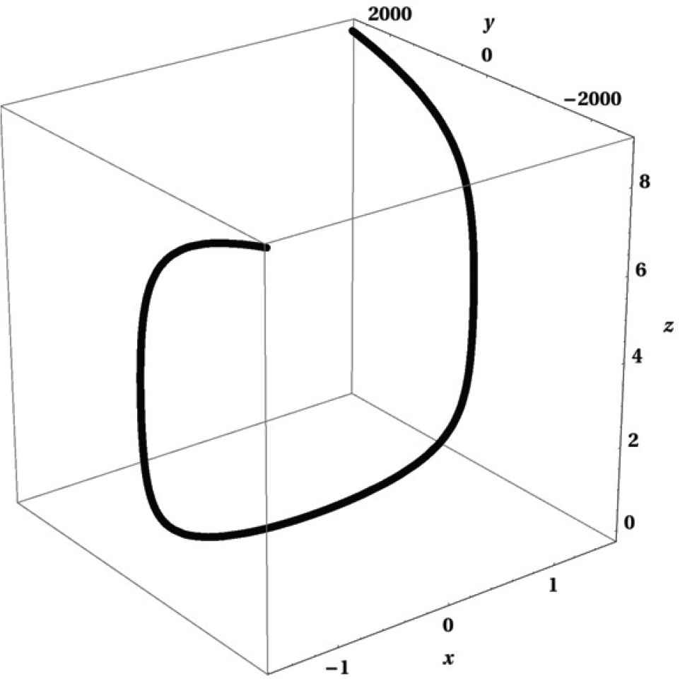
If we assume b=q2, then from (4.11) we have

z″−(a−q2)2e−2z−q2(a−q2)e−z=0.(4.17)

The solution of this equation is

z(s)=−ln[(b−q2)(1+q22coshs+q2)].

Further, from (4.7) and (4.10) it follows

x(s)=2(2a−2q)2+q2⋅sinhs(q+2+q2⋅coshs),y(s)=q⋅(2a−2q)4(q⋅s+2+q2⋅sinhs).

Particularly, for q = 0 we obtain geodesic line in xz-plane.

Figure 3 shows the magnetic curve for a = 1, q=12, s ∈ [−10, 10].

Remark 4.2 (Magnetic Jacobi fields).

Adachi [1] and Gouda [11] obtained the second variational formula of the Landau-Hall functional:

d2dε2|ε=0LH(γε)=−∫0ℓg(Jq,F(V),V(s))ds,

where Jq,F is an operator acting on the space Γ(γ*TM) of all vector fields along γ defined by

Jq,F(W)=∇γ′∇γ′W+R(W,γ′)γ′−qφ(∇γ′W)−q(∇Wφ)γ′.

A vector field W(s) along γ is said to be a magnetic Jacobi field if it satisfies Jq,F(W)=0. Detailed study on magnetic Jacobi fields gives us insight on how small variations in the initial conditions affect the evolution of magnetic curves. In this direction, Adachi obtained the comparison theorem for magnetic curves on Kähler manifold whose Lorentz force is a complex structure [1]. Gouda [11, 12] studied magnetic Jacobi fields on Riemannian 2-manifolds equipped with compatible Kähler structure. The parallelism of the complex structure (the Lorentz force) is crucial in these works.

In case (M, g)= Sol₃, the sectional curvature function can have both signs. In addition the Lorentz force φ is non-parallel. Thus the behavior of magnetic Jacobi fields along contact magnetic curves in Sol₃ appears complicated. This will be addressed in future work.

Acknowledgments

The second named author is partially supported by JSPS Kakenhi 15K048340. The authors would like to thank the referee for her/his careful reading of the manuscript and many suggestions for improving this article.

References

[1]T. Adachi, A comparison theorem on magnetic Jacobi ﬁelds, Proc. Edinburgh Math. Soc., Vol. 40, 1997, pp. 293-308.

[2]V. I. Arnold, Some remarks on ﬂows of line elements and frames, Sov. Math. Dokl., Vol. 2, 1961, pp. 562-564.

[3]D. E. Blair, Riemannian Geometry of Contact and Symplectic Manifolds, Progress in Math, Birkhäuser, Basel, Vol. 203, 2002.

[4]D. E. Blair and D. Perrone, Conformally Anosov ﬂows in contact metric geometry, Balkan J. Geom. Appl., Vol. 3, No. 2, 1998, pp. 33-46.

[5]A. Bölcskei and B. Szilágyi, Visualization of curves and spheres in Sol geometry, KoG, Vol. 10, 2006, pp. 27-32.

[6]A. Bölcskei and B. Szilágyi, Frenet formulas and geodesics in Sol geometry, Beit. Alg. Geom, Vol. 48, No. 2, 2007, pp. 411-421.

[7]J. L. Cabrerizo, M. Fernández, and J. S. Gómez, The contact magnetic ﬂow in 3D Sasakian manifolds, J. Phys. A: Math. Theor., Vol. 42, No. 19, 2009, pp. 10. 195201

[8]S. L. Druţă-Romaniuc, J. Inoguchi, M. I. Munteanu, and A. I. Nistor, Magnetic curves in Sasakian manifolds, J. Nonlinear Math. Phys., Vol. 22, No. 3, 2015, pp. 428-447.

[9]Z. Erjavec, On a certain class of Weingarten surfaces in Sol space, Int. J. Appl. Math., Vol. 28, No. 5, 2015, pp. 507-514.

[10]V. L. Ginzburg, A charge in a magnetic ﬁeld: Arnold’s problems 1981-9, 1982-24, 1984-4, 1994-14, 1994-35, 1996-17,1996-18, V.I. Arnold (editor), Arnold’s problems, Springer-Verlag and Phasis, 2004, pp. 395-401.

[11]N. Gouda, Magnetic ﬂows of Anosov type, Tohoku Math. J., Vol. 49, 1997, pp. 165-183.

[12]N. Gouda, The theorem of E. Hopf under uniform magnetic ﬁelds, J. Math. Soc. Japan, Vol. 50, No. 3, 1998, pp. 767-779.

[13]J. Inoguchi, Minimal surfaces in 3-dimensional solvable Lie groups, Chinese Ann. Math. B., Vol. 24, 2003, pp. 73-84.

[14]J. Inoguchi, On homogeneous contact 3-manifolds, Bull. Fac. Edu. Utsunomiya Univ. Sect. 2., Vol. 59, 2009, pp. 1-12.

[15]J. Inoguchi and S. Lee, A Weierstrass type representation for minimal surfaces in Sol, Proc. Amer. Math. Soc., Vol. 146, 2008, pp. 2209-2216.

[16]R. López and M. I. Munteanu, On the geometry of constant angle surfaces in Sol3, Kyushu J. Math., Vol. 65, 2011, pp. 237-249.

[17]R. López and M. I. Munteanu, Surfaces with constant mean curvature in Sol geometry, Differential. Geom. Appl., Vol. 29, 2011, pp. 238-245.

[18]R. López and M. I. Munteanu, Minimal translation surfaces in Sol3, J. Math. Soc. Japan, Vol. 64, No. 3, 2012, pp. 985-1003.

[19]R. Lutz, Sur quelques propriétés des formes différentielles en dimension trois, Thése, Strasbourg, 1971.

[20]J. Martinet, Formes de contact sur les variétés de dimension 3, Proc. Liverpool Singularity Sympos. II, Lecture Notes in Math, Vol. 209, 1971, pp. 142-163.

[21]J. Milnor, Curvatures of left invariant metrics on Lie groups, Adv. Math., Vol. 21, 1976, pp. 293-329.

[22]Y. Mitsumatsu, Anosov ﬂows and non-Stein symplectic manifolds, Ann. Inst. Fourier, Vol. 45, No. 5, 1995, pp. 1407-1421.

[23]M. I. Munteanu and A. I. Nistor, On some closed magnetic curves on a 3-torus, Math. Phys. Anal. Geom., Vol. 20, No. 8, 2017, pp. 13.

[24]D. Perrone, Homogeneous contact Riemannian three-manifolds, Illinois J. Math., Vol. 13, 1997, pp. 243-256.

[25]T. Sunada, Magnetic ﬂows on a Riemann surface, Proc. KAIST Mathematics Workshop: Analysis and Geometry, KAIST, Taejeon, Korea, 1993, pp. 93-108.

[26]W. M. Thurston, S. Levy (editor), Three-dimensional Geometry and Topology I, Princeton Math. Series., Vol. 35, 1997.

[27]W. M. Thurston and H. E. Winkelnkemper, On the existence of contact forms, Proc. Amer. Math. Soc., Vol. 52, No. 1, 1975, pp. 345-347.

[28]M. Troyanov, L’horizon de SOL, Expo. Math., Vol. 16, 1998, pp. 441-479.

[29]M. S. Wo, R. U. Gobithaasan, and K. T. Miura, Log-aesthetic magnetic curves and their application for CAD systems, Math. Probl. Eng., 2014, pp. 16. Article ID 504610 (2014)

[30]L. Xu and D. Mould, Magnetic curves: Curvature-controlled aesthetic curves using magnetic fields, O. Deussen and P. Hall (editors), Computational Aesthetics in Graphics, Visualization and Imaging, Victoria, British Columbia, Canada, 2009, pp. 1-8.

<Previous Article In Issue

Download article (PDF)

Next Article In Issue>

Journal: Journal of Nonlinear Mathematical Physics
Volume-Issue: 25 - 2
Pages: 198 - 210
Publication Date: 2021/01/06
ISSN (Online): 1776-0852
ISSN (Print): 1402-9251
DOI: 10.1080/14029251.2018.1452670 How to use a DOI?
Open Access: This is an open access article distributed under the CC BY-NC 4.0 license (http://creativecommons.org/licenses/by-nc/4.0/).

Cite this article

ris enw bib

TY  - JOUR
AU  - Zlatko Erjavec
AU  - Jun-ichi Inoguchi
PY  - 2021
DA  - 2021/01/06
TI  - Magnetic curves in Sol₃
JO  - Journal of Nonlinear Mathematical Physics
SP  - 198
EP  - 210
VL  - 25
IS  - 2
SN  - 1776-0852
UR  - https://doi.org/10.1080/14029251.2018.1452670
DO  - 10.1080/14029251.2018.1452670
ID  - Erjavec2021
ER  -

download .riscopy to clipboard

Journal of Nonlinear Mathematical Physics

Magnetic curves in Sol3

Introduction

1. Magnetic curves

Remark 1.1.

2. Contact structures

Remark 2.1.

Remark 2.2.

3. Invariant contact structure on Sol3

3.1. Model of the Sol3 space

3.2. Invariant contact structure on Sol3

Remark 3.1.

4. Magnetic curves in Sol 3

4.1. Contact magnetic fields

4.2. Magnetic curve equation

Remark 4.1.

Theorem 4.1.

Example 1

Example 2

Example 3

Example 4

Remark 4.2 (Magnetic Jacobi fields).

Acknowledgments

References

Cite this article

Magnetic curves in Sol₃

3. Invariant contact structure on Sol₃

3.1. Model of the Sol₃ space

3.2. Invariant contact structure on Sol₃

4. Magnetic curves in Sol ₃