Journal of Nonlinear Mathematical Physics

Volume 25, Issue 1, February 2018, Pages 136 - 165

Initial-boundary value problem for the two-component Gerdjikov-Ivanov equation on the interval

Authors
Qiaozhen Zhu, Jian Xu, Engui Fan*
School of Mathematical Sciences, Fudan University, NO.220 Handan Road, Shanghai, 200433, People’s Republic of China,qiaozhenzhu13@fudan.edu.cn
College of Science, University of Shanghai for Science and Technology, NO.334 Jungong Road, Shanghai 200093, People’s Republic of China,jianxu@usst.edu.cn
School of Mathematical Sciences, Fudan University, NO.220 Handan Road, Shanghai, 200433, People’s Republic of China,faneg@fudan.edu.cn
*Corresponding author.
Corresponding Author
Engui Fan
Received 12 October 2017, Accepted 28 October 2017, Available Online 6 January 2021.
DOI
10.1080/14029251.2018.1440747How to use a DOI?
Keywords
Two-component Gerdjikov-Ivanov equation; initial-boundary value problem; Fokas unified method; Riemann-Hilbert problem
Abstract

In this paper, we apply Fokas unified method to study initial-boundary value problems for the two-component Gerdjikov-Ivanov equation formulated on the finite interval with 3×3 Lax pairs. The solution can be expressed in terms of the solution of a 3×3 Riemann-Hilbert problem. The relevant jump matrices are explicitly given in terms of three matrix-value spectral functions s (λ), S (λ) and SL(λ), which arising from the initial values at t = 0, boundary values at x = 0 and boundary values at x = L, respectively. Moreover, The associated Dirichlet to Neumann map is analyzed via the global relation. The relevant formulae for boundary value problems on the finite interval can reduce to ones on the half-line as the length of the interval tends to infinity.

Copyright
© 2018 The Authors. Published by Atlantis and Taylor & Francis
Open Access
This is an open access article distributed under the CC BY-NC 4.0 license (http://creativecommons.org/licenses/by-nc/4.0/).

1. Introduction

The Gerdjikov-Ivanov (GI) equation takes in the form [10]

qt=iqxx+q2q¯x+i2q3q¯2.(1.1)
In these years, there has been much work on the GI equation, including Hamiltonian structures [2], Darboux transformation [3], rouge wave and breather soliton [19], algebro-geometric solutions [11], envelope bright and dark soliton solution [17]. Recently, Zhang, Cheng and He obtained the N-soliton solutions with Riemann-Hilbert method about the two-component (2-GI) equation [22]
{q1t=iq1xx+q1(q1q¯1x+q2q¯2x)+i2q1(|q1|4+|q2|4)+i|q1q2|2q1,q2t=iq2xx+q2(q1q¯1x+q2q¯2x)+i2q2(|q1|4+|q2|4)+i|q1q2|2q2.(1.2)

In 1997, Fokas announced the unified transform for the analysis of initial boundary value (IBV) problems for linear and nonlinear integrable PDEs [4]. The Fokas method was usually used to analyze the IBV problem for integrable PDEs with 2 × 2 Lax pair on the half-line and the finite interval, such as nonlinear Schröding equation [5, 6], sine-Gordon equation [7,15], KdV equation [8], mKdV equation [1, 9], derivative nonlinear Schröding equation [12]. In 2012, Lenells extended this method to the IBV problem of integrable systems with 3 × 3 Lax pair on the half-line [13]. After that, several important integrable equations with 3 × 3 Lax pair have been investigated, including Degasperis-Procesi [14], Sasa-satuma [18]. However, there has been still less work on the IBV problems on the finite interval of integrable equations with 3 × 3 Lax pair except to the two-component NLS [20], general coupled NLS [16] and the integrable spin-1 Gross-Pitaevskii [21] equations.

In this paper, we apply Fokas method to consider 2-GI equation with the following initial boundary value data:

Initial value:q1(x,t=0)=q10(x),q2(x,t=0)=q20(x),Dirichlet boundary value:q1(x=0,t)=g01(t),q1(x=L,t)=f01(t),q2(x=0,t)=g02(t),q2(x=L,t)=f02(t),Neumann boundary value:q1x(x=0,t)=g11(t),q1x(x=L,t)=f11(t),q2x(x=0,t)=g12(t),q2x(x=L,t)=f12(t),(1.3)
where q1(x, t) and q2(x, t) are complex-valued functions of (x, t) ∈ Ω, and Ω denotes the finite interval domain
Ω={(x,t)0xL,0tT},
here L > 0 is a positive fixed constant and T > 0 being a fixed final time.

Comparing with two-component NLS equation [20], the IBV problem of the 2-GI equation (1.2) also presents some distinctive features in the use of Fokas method: (i) The order of spectral variable k in the Lax pair (2.1) is higher than that of 2-NLS equation. In order to make the results on the interval reduce to the ones on the half-line, we should first introduce transformation ψ(x,t,k)=k12Λϕ(x,t,k)k12Λ so that the Lax pairs are even functions of k. (ii) The 2-GI equation admits a generalized Wadati-Konno-Ichikawa (WKI) type Lax pair, which admits a gauge transformation to AKNS-type Lax pair, but this gauge transformation can not be used to analyze the IBV problem by mapping it into 2-NLS equation. We need to introduce a matrix-value function G(x, t) to transform the WKI-type Lax pair into AKNS-type Lax pair.

Organization of this paper is as follows. In the following section 2, we perform the spectral analysis of the associated Lax pair for the 2-GI equation (1.2). In the section 3, we give the corresponding matrix RH problem associated with the IBV problem of 2-GI equation. In section 4, we get the map between the Dirichlet and the Neumann boundary problem through analysising the global relation. Especially, the relevant formulae for boundary value problems on the finite interval can reduce to ones on the half-line as the length of the interval approaches to infinity.

2. Spectral analysis

2.1. Lax pair

The 2-GI equation admits a 3 × 3 Lax pair [22]

ψx+ik2Λψ=U1ψ,(2.1a)
ψt+2ik4Λψ=U2ψ,(2.1b)
where ψ(x, t, k) is a 3 × 3 – matrix valued eigenfunction, k ∈ ℂ is the spectral parameter, and U1(x, t), U2(x, t) are 3 × 3 – matrix valued functions given by
U1=kQΛ+i2Q2Λ,U2=2k3QΛ+ik2ΛQ2+ikQx12[Qx,Q]+i4Q4Λ,(2.2)
Λ=(100010001),Q=(0q1q2q¯100q¯200).(2.3)

There are both odd power and even power of k in the Lax pair (2.1), to make (2.1) are even functions of k for analyzing the large L limit, we introduce a transformation

ψ(x,t,k)=k12Λϕ(x,t,k)k12Λ,(2.4)
and get an equivalent Lax pair
ϕx+ik2Λϕ=U˜1ϕ,(2.5a)
ϕt+2ik4Λϕ=U˜2ϕ,(2.5b)
where
U˜1=Q1Λk2Q2Λ+i2Q2Λ,U˜2=2k4Q2Λ+k2(iΛQ2+iQ2x2Q1Λ)+(iQ1x12[Qx,Q]+i4Q4Λ),(2.6)
Q1=(0q1q2000000),Q2=(000q¯100q¯200),Q=Q1+Q2.(2.7)

Let λ = k2, Lax pair (2.5) becomes

ϕx+iλΛϕ=U˜1ϕ,(2.8a)
ϕt+2iλ2Λϕ=U˜2ϕ,(2.8b)
where U˜1,U˜2 are given by (2.6) with k2 replaced with λ.

2.2. The closed one-form

Defining a 3 × 3 matrix-value function

G(x,t)=(10012iq¯11012iq¯201),(2.9)
and making a transformation
ϕ(x,t,k)=G(x,t)μ(x,t,k)eiλΛx2iλ2Λt,(2.10)
then we get a new Lax pair for μ(x, t, λ)
μx+iλ[Λ,μ]=V1μ,(2.11a)
μt+2iλ2[Λ,μ]=V2μ,(2.11b)
where
V1=G1(Q1Λ+i2Q2Λ)GG1Gx,(2.12a)
V2=λG1(iΛQ2+iQ2x2Q1Λ)G+G1(iQ1x12[Qx,Q]+i4Q4Λ)GG1Gt.(2.12b)

Letting A^ denotes the operators which acts on a 3 × 3 matrix X by A^X=[A,X], then the equations (2.11) can be rewritten in a differential form

d(e(iλx+2iλ2t)Λ^μ)=W,(2.13)
where the closed one-form W(x, t, k) is defined by
W=e(iλx+2iλ2t)Λ^(V1dx+V2dt)μ.(2.14)

2.3. The eigenfunctions μj’s

We define four eigenfunctions {μj}14 of (2.11) by the Volterra integral equations

μj(x,t,k)=I+γje(iλx+2iλ2t)Λ^Wj(x,t,k).j=1,2,3,4.(2.15)
where Wj is given by (2.14) with μ replaced by μj, and the contours {γj}14 can be given by the following inequalities ( see Figure 1):
γ1:xx0,tt0,γ2:xx0,tt0,γ3:xx0,tt0,γ4:xx0,tt0.(2.16)
and the matrix equation (2.15) involves the exponentials
[μj]1:e2iλ(xx)+4iλ2(tt),e2iλ(xx)+4iλ2(tt)[μj]2:e2iλ(xx)4iλ2(tt),[μj]3:e2iλ(xx)4iλ2(tt).(2.17)
from which, we find that the functions {μj}14 are bounded and analytic for λ ∈ ℂ such that λ belongs to
μ1:(D2,D3,D3),μ2:(D1,D4,D4),μ3:(D3,D2,D2),μ4:(D4,D1,D1),(2.18)
where {Dn}14 denote four open, pairwisely disjoint subsets of the complex λ – plane showed in Figure 2.

And the sets {Dn}14 admit the following properties:

D1={kRel1>Rel2=Rel3,Rez1>Rez2=Rez3},D2={kRel1>Rel2=Rel3,Rez1<Rez2=Rez3},D3={kRel1<Rel2=Rel3,Rez1>Rez2=Rez3},D4={kRel1<Rel2=Rel3,Rez1<Rez2=Rez3},
where li(λ) and zi(λ) are the diagonal entries of matrices Λ and 22Λ, respectively.

Fig. 1.

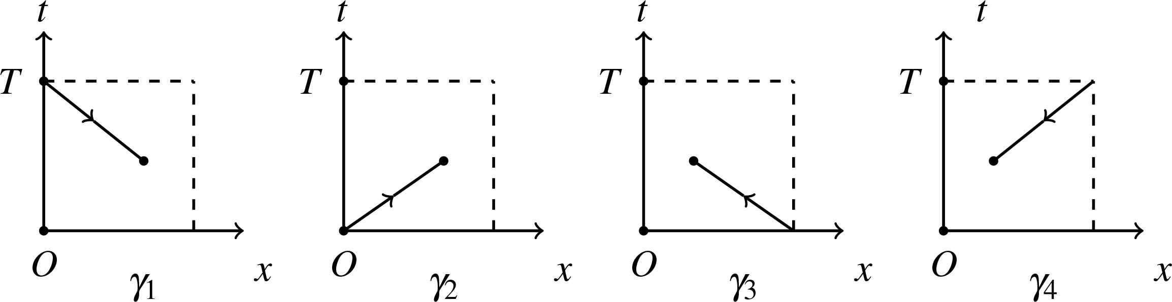
The four contours γ1, γ2, γ3 and γ4 in the (x, t) – domain.

Fig. 2.

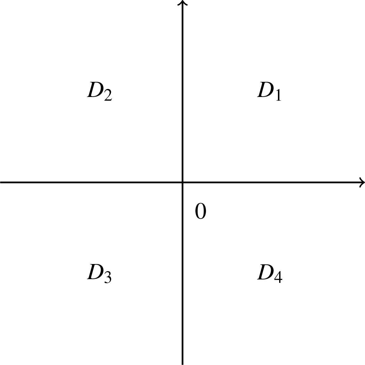
The sets Dn, n = 1,…,4, which decompose the complex λ-plane.

2.4. The spectral functions Mn’s

For each n = 1, …, 4, a solution Mn(x, t, λ) of (2.11) can be defined by the following system of integral equations:

(Mn)ij(x,t,λ)=δij+γijn(e(iλx+2iλ2t)Λ^Wn(x,t,λ))ij,λDn,i,j=1,2,3.(2.19)
where Wn is given by (2.14) with μ replaced with Mn, and the contours γijn,n=1,,4,i,j=1,2,3 are defined by
γijn={γ1 if Reli(λ)<Relj(λ) and Rezi(λ)Rezj(λ),γ2 if Reli(λ)<Relj(λ) and Rezi(λ)<Rezj(λ),γ3 if Reli(λ)Relj(λ) and Rezi(λ)Rezj(λ),γ4 if Reli(λ)Relj(λ) and Rezi(λ)Rezj(λ), for λDn.(2.20)
Here, we make a distinction between the contours γ3 and γ4 as follows,
γijn={γ3, if Π1i<j3(Reli(λ)Relj(λ))(Rezi(λ)Rezj(λ))<0,γ4, if Π1i<j3(Reli(λ)Relj(λ))(Rezi(λ)Rezj(λ))>0.(2.21)
The rule chosen in the produce is if lm = ln, m may not equals n, we just choose the subscript is smaller one.

According to the definition of the γn, one find that

γ1=(γ4γ4γ4γ2γ4γ4γ2γ4γ4)γ2=(γ3γ3γ3γ1γ3γ3γ1γ3γ3)γ3=(γ3γ1γ1γ3γ3γ3γ3γ3γ3)γ4=(γ4γ2γ2γ4γ4γ4γ4γ4γ4).(2.22)

The following proposition ascertains that the Mn’s defined in this way have the properties required for the formulation of a Riemann-Hilbert problem.

Proposition 2.1.

For each n = 1,…,4, the function Mn(x, t, λ) is well-defined by equation (2.19) for λD¯n and (x,t)Ω. Moreover, Mn admits a bounded and contious extension to D¯n and

Mn(x,t,λ)=I+O(1λ),λ,λDn.(2.23)

Proof. Analogous to the proof provided in [13] □

Remark 2.1.

Of course, for any fixed point (x, t), Mn is bounded and analytic as a function of kDn away from a possible discrete set of singularities {kj} at which the Fredholm determinant vanishes. The bounedness and analyticity properties are established in appendix B in [13]. □

2.5. The jump matrices

The spectral functions {Sn(λ)}14 can be defined by

Sn(λ)=Mn(0,0,λ),λDn,n=1,,4.(2.24)
Let M denote the sectionally analytic function on the Riemann λ – plane which equals Mn for λDn. Then M satisfies the jump conditions
Mn=MmJm,n,kD¯nD¯m,n,m=1,,4,nm,(2.25)
where the jump matrices Jm, n(x, t, λ) are given by
Jm,n=e(iλx+2iλ2t)Λ^(Sm1Sn).(2.26)

2.6. The adjugated eigenfunctions

As the expressions of Sn(λ) will involve the adjugate matrix of {s(λ), S(λ), SL(λ)} defined in the next subsection. We will also need the analyticity and boundedness of the the matrices {μj(x,t,λ)}14. We recall that the adjugate matrix XA of a 3 × 3 matrix X is defined by

XA=(m11(X)m12(X)m13(X)m21(X)m22(X)m23(X)m31(X)m32(X)m33(X)),
where mi j(X) denote the (i j) th minor of X.

It follows from (2.11) that the adjugated eigenfunction μA satisfies the Lax pair

{μxAiλ[Λ,μA]=V1TμA,μtA2iλ2[Λ,μA]=V2TμA.(2.27)
where VT denotes the transform of a matrix V. Thus, the eigenfunctions {μjA}14 are solutions of the integral equations
μjA(x,t,λ)=Iγjeiλ(xx)+2iλ2(tt)Λ^(V1Tdx+V2Tdt)μjA,j=1,2,3.(2.28)
Then we can get the following analyticity and boundedness properties:
μ1A:(D3,D2,D2),μ2A:(D4,D1,D1),μ3A:(D2,D3,D3),μ4A:(D1,D4,D4).(2.29)

2.7. Symmetries

We will show that the eigenfunctions μj(x, t, k) satisfy an important symmetry.

Proposition 2.2.

The eigenfunction ψ(x, t, k) of the Lax pair (2.1) satisfies the following symmetry:

ψ1(x,t,k)=ψ(x,t,k¯)¯T=Λψ(x,t,k)Λ,(2.30)
here the superscript T denotes a matrix transpose.

Proof. The matrices U(x, t, k) and V(x, t, k) in the Lax pair (2.1) written in the form

ψx=Uψ,ψt=Vψ,
satisfy the following symmetry relations
U(x,t,k)T=U(x,t,k¯)¯,V(x,t,k)T=V(x,t,k¯)¯,(2.31)
and
U(x,t,k)=ΛU(x,t,k)Λ,V(x,t,k)=ΛV(x,t,k)Λ.(2.32)
In turn, relations (2.31) and (2.32) imply
ψxA(x,t,k)=U(x,t,k¯)¯ψA(x,t,k),ψtA(x,t,k)=V(x,t,k¯)¯ψA(x,t,k),(2.33)
and
ψxA(x,t,k)=ΛUT(x,t,k)ΛψA(x,t,k),ψtA(x,t,k)=ΛV(x,t,k)ΛψA(x,t,k).(2.34)

Remark 2.2.

From proposition 2.3, one can show that the eigenfunctions μj(x, t, λ) of Lax pair equations (2.11) satisfy the same symmetry.

2.8. The Jm, n’s computation

Let us define the 3 × 3 – matrix value spectral functions s(λ), S(λ) and SL(λ) by

μ3(x,t,λ)=μ2(x,t,λ)e(iλx+2iλ2t)Λ^s(λ),(2.35a)
μ1(x,t,λ)=μ2(x,t,λ)e(iλx+2iλ2t)Λ^S(λ),(2.35b)
μ4(x,t,λ)=μ3(x,t,λ)e(iλ(xL)+2iλ2t)Λ^SL(λ),(2.35c)
Thus,
s(λ)=μ3(0,0,λ),(2.36a)
S(λ)=μ1(0,0,λ)=e2iλ2TΛ^μ21(0,T,λ),(2.36b)
SL(λ)=μ4(L,0,λ)=e2iλ2TΛ^μ31(L,T,λ),(2.36c)
And we can deduce from the properties of μj and μjA that {s(λ), S(λ), SL(λ)} and {sA(λ),SA(λ),SLA(λ)} have the following boundedness properties:
s(λ):(D3D4,D1D2,D1D2),S(λ):(D2D4,D1D3,D1D3),SL(λ):(D2D4,D1D3,D1D3),sA(λ):(D1D2,D3D4,D3D4),SA(λ):(D1D3,D2D4,D2D4),SLA(λ):(D1D3,D2D4,D2D4).
Moreover,
Mn(x,t,λ)=μ2(x,t,λ)e(iλx+2iλ2t)Λ^Sn(λ),λDn.(2.37)

Proposition 2.3.

The Sn can be expressed in terms of the entries of s(λ), S(λ) and SL(λ) as follows:

S1=(1m11(A)A12A130A22A230A32A33),S2=(S11(STsA)11s12s13S21(STsA)11s22s23S31(STsA)11s32s33),(2.38a)
S3=(S11m33(s)m21(S)m23(s)m31(S)(sTSA)11m32(s)m21(S)m22(s)m31(S)(sTSA)11S21m33(s)m11(S)m13(s)m31(S)(sTSA)11m32(s)m11(S)m12(s)m31(S)(sTSA)11S31m23(s)m11(S)m13(s)m21(S)(sTSA)11m22(s)m11(S)m12(s)m21(S)(sTSA)11),(2.38b)
S4=(A1100A21m33(A)A11m32(A)A11A31m23(A)A11m22(A)A11).
where A=(Aij)i,j=13 is a 3 × 3 matrix, which is defined as A=s(λ)eiλLΛ^SL(λ). And the functions
(STsA)11=S11m11(s)S21m21(s)+S31m31(s),(sTSA)11=s11m11(S)s21m21(S)+s31m31(S).

Proof. Firstly, we define Rn(λ), Tn(λ) and Qn(λ) as follows:

Rn(λ)=e2iλ2TΛ^Mn(0,T,λ),(2.39a)
Tn(λ)=eiλLΛ^Mn(L,0,λ),(2.39b)
Qn(λ)=e(iλL+2iλ2T)Λ^Mn(L,T,λ).(2.39c)
Then, we have the following relations:
{Mn(x,t,λ)=μ1(x,t,λ)e(iλx+2iλ2t)Λ^Rn(λ),Mn(x,t,λ)=μ2(x,t,λ)e(iλx+2iλ2t)Λ^Sn(λ),Mn(x,t,λ)=μ3(x,t,λ)e(iλx+2iλ2t)Λ^Tn(λ),Mn(x,t,λ)=μ4(x,t,λ)e(iλx+2iλ2t)Λ^Qn(λ).(2.40)

The relations (2.40) imply that

s(λ)=Sn(λ)Tn1(λ),S(λ)=Sn(λ)Rn1(λ),A(λ)=Sn(λ)Qn1(λ),(2.41)
These equations constitute a matrix factorization problem which, given {s(λ), S(λ), SL(λ)} can be solved for the {Rn, Sn, Tn, Qn}. Indeed, the integral equations (2.19) together with the definitions of {Rn, Sn, Tn, Qn} imply that
{(Rn(λ))ij=0 if γijn=γ1,(Sn(λ))ij=0 if γijn=γ2,(Tn(λ))ij=δij if γijn=γ3,(Qn(λ))ij=δij if γijn=γ4.(2.42)
It follows that (2.41) are 27 scalar equations for 27 unknowns. By computing the explicit solution of this algebraic system, we arrive at (2.38). □

Remark 2.3.

Due to our symmetry, see Lemma 2.30, the representation of the functions Sn(λ) can be become simple. It leads to much more simple to compute the jump matrices Jm, n(x, t, λ).

2.9. The residue conditions

Since μ2 is an entire function, it follows from (2.37) that M can only have sigularities at the points where the Sn s have singularities. We denote the possible zeros by {λj}1N and assume they satisfy the following assumption. We assume that

  • m11()(λ) has n0 possible simple zeros in D1 denoted by {λj}1n0;

  • (ST sA)11(k) has n1n0 possible simple zeros in D2 denoted by {λj}n0+1n1;

  • (sT SA)11(k) has n2n1 possible simple zeros in D3 denoted by {λj}n1+1n2;

  • 11(k) has Nn2 possible simple zeros in D4 denoted by {λj}n2+1N;

and that none of these zeros coincide. Moreover, we assume that none of these functions have zeros on the boundaries of the Dns. We determine the residue conditions at these zeros in the following:

Proposition 2.4.

Let {Mn}14 be the eigenfunctions defined by (2.19) and assume that the set {λj}1N of singularities are as the above assumption. Then the following residue conditions hold:

Resλ=λj[M]1=A33(λj)[M(λj)]2A23(λj)[M(λj)]3m˙11(A)(λj)m21(A)(λj)e2θ(λj),1jn0,λjD1(2.43a)
Resλ=λj[M]1=S21(λj)s33(λj)S31(λj)s23(λj)(STsA)11(λj)m11(λj)e2θ(λj)[M(λj)]2+S31(λj)s22(λj)S21(λj)s32(λj)(STsA)11(λj)m11(λj)e2θ(λj)[M(λj)]3 n0+1jn1,λjD2,(2.43b)
Resλ=λj[M]2=m33(s)(λj)m21(S)(λj)m23(s)(λj)m31(S)(λj)(sTSA)11(λj)s11(λj)e2θ(λj)[M(λj)]1 n1+1jn2,λjD3,(2.43c)
Resλ=λj[M]3=m32(s)(λj)m21(S)(λj)m22(s)(λj)m31(S)(λj)(sTSA)11(λj)s11(λj)e2θ(λj)[M(λj)]1 n1+1jn2,λjD3.(2.43d)
Resλ=λj[M]2=m33(A)(λj)A˙11(λj)A21(λj)e2θ(λj)[M(λj)]1,n2+1jN,λjD4.(2.43e)
Resλ=λj[M]3=m22(A)(λj)A.11(λj)A21(λj)e2θ(λj)[M(λj)]1,n2+1jN,λjD4.(2.43f)
where f˙=dfdλ, and θ is defined by
θ(x,t,λ)=iλx+2iλ2t.(2.44)

Proof. We will prove (2.43a),(2.43c), the other conditions follow by similar arguments. Equation (2.37) implies the relation

M1=μ2e(iλx+2iλ2t)Λ^S1,(2.45a)
M3=μ2e(iλx+2iλ2t)Λ^S3,(2.45b)

In view of the expressions for S1 and S3 given in (2.38), the three columns of (2.45a) read:

[M1]1=[μ2]11m11(A),(2.46a)
[M1]2=[μ2]1e2θA12+[μ2]2A22+[μ2]3A32,(2.46b)
[M1]3=[μ2]1e2θA13+[μ2]2A23+[μ2]3A33.(2.46c)
while the three columns of (2.45b) read:
[M3]1=[μ2]1s11+[μ2]2s21e2θ+[μ2]3s31e2θ(2.47a)
[M3]2=[μ2]1m33(s)m21(S)m23(s)m31(S)(sTSA)11e2θ+[μ2]2m33(s)m11(S)m13(s)m31(S)(sTSA)11+[μ2]3m23(s)m11(S)m13(s)m21(S)(sTSA)11(2.47b)
[M3]3=[μ2]1m32(s)m21(S)m22(s)m31(S)(sTSA)11e2θ+[μ2]2m32(s)m11(S)m12(s)m31(S)(sTSA)11+[μ2]3m22(s)m11(S)m12(s)m21(S)(sTSA)11.(2.47c)

We first suppose that λjD1 is a simple zero of m11()(λ). Solving (2.46b) and (2.46c) for [μ2]1,[μ2]3 and substituting the result in to (2.46a), we find

[M1]1=A33[M1]2A32[M1]3m11(A)m21(A)e2θ[μ2]2m21(A)e2θ.
Taking the residue of this equation at λj, we find the condition (2.43a) in the case when λjD1.

In order to prove (2.43c), we solve (2.47a) for [μ2]1, then substituting the result into (2.47b) and (2.47c), we find

[M3]2=m33(s)s11[μ2]2+m23(s)s11[μ2]3+m33(s)m21(S)m23(s)m31(S)(sTS˙A)11s11e2θ[M3]1,(2.48a)
[M3]3=m32(s)s11[μ2]2+m22(s)s11[μ2]3+m32(s)m21(S)m22(s)m31(S)(sTS˙A)11s11e2θ[M3]1.(2.48b)
Taking the residue of this equation at λj, we find the condition (2.43c) in the case when λjD3. □

2.10. The global relation

The spectral functions S(λ), SL(λ) and s(λ) are not independent but satisfy an important relation. Indeed, it follows from (2.35) that

μ1(x,t,λ)e(iλx+2iλ2t)Λ^{S1(λ)s(λ)eiλLΛ^SL(λ)}=μ4(x,t,λ).(2.49)
Since μ1(0, T, λ) = !!!x1D540;, evaluation at (0, T) yields the following global relation:
S1(λ)s(λ)eiλLΛ^SL(λ)=e2iλ2TΛ^c(T,λ),(2.50)
where c(T, λ) = μ4(0, T, λ)

3. The Riemann-Hilbert problem

The sectionally analytic function M(x, t, λ) defined in section 2 satisfies a Riemann-Hilbert problem which can be formulated in terms of the initial and boundary values of q1(x, t) and q2(x, t). By solving this Riemann-Hilbert problem, the solution of (1.2) can be recovered for all values of x, t.

Theorem 3.1.

Suppose that q1(x, t) and q2(x, t) are a pair of solutions of (1.2) in the interval domain Ω. Then q1(x, t) and q2(x, t) can be reconstructed from the initial value {q10(x), q20(x)} and boundary values {g01(t), g02(t), g11(t), g12(t)},{f01(t), f02(t), f11(t), f12(t)} defined as follows,

q10(x)=q1(x,t=0),q20(x)=q2(x,t=0),g01(t)=q1(x=0,t),g02(t)=q2(x=0,t),f01(t)=q1(x=L,t),f02(t)=q2(x=L,t),g11(t)=q1x(x=0,t),g12(t)=q2x(x=0,t),f11(t)=q1x(x=L,t),f12(t)=q2x(x=L,t).(3.1)

Use the initial and boundary data to define the jump matrices Jm, n(x, t, λ) in terms of the spectral functions s(λ) and S(λ), SL(λ) by equation (2.35).

Assume that the possible zeros {λj}1N of the functions m11()(λ),(ST sA)11(λ),(sT SA)11(λ) and11(λ) are as the assumption in subsection 2.8.

Then the solution {q1(x, t), q2(x, t)} is given by

q1(x,t)=2ilimλ(λM(x,t,λ))12,q2(x,t)=2ilimλ(λM(x,t,λ))13.(3.2)
where M(x, t, λ) satisfies the following 3 × 3 matrix Riemann-Hilbert problem:
  • M is sectionally meromorphic on the Riemann λsphere with jumps across the contours D¯nD¯m,n,m=1,,4, see Figure 2.

  • Across the contours D¯nD¯m, M satisfies the jump condition

    Mn(x,t,λ)=Mm(x,t,λ)Jm,n(x,t,λ),λD¯nD¯m,n,m=1,2,3,4.(3.3)

  • M(x,t,λ)=I+O(1λ), λ.

  • The residue condition of M is showed in Proposition 2.4.

Proof. It only remains to prove (3.2) and this equation follows from the large λ asymptotics of the eigenfunctions. □

4. Non-linearizable Boundary Conditions

A key difficulty of initial-boundary value problems is that some of the boundary values are unkown for a well-posed problem. While we need all boundary values to define the spectral functions S(λ) and SL(λ), and hence for the formulation of the Riemann-Hilbert problem. Our main result, Theorem 4.3, expresses the unknown boundary data in terms of the prescribed boundary data and the initial data in terms of the solution of a system of nonlinear integral equations.

4.1. Asymptotics

An analysis of (2.11) shows that the eigenfunctions {μj}14 have the following asymptotics as λ → ∞ :

μj(x,t,λ)=I+1λ(μ11(1)μ12(1)μ13(1)μ21(1)μ22(1)μ23(1)μ31(1)μ32(1)μ33(1))+1λ2(μ11(2)μ12(2)μ13(2)μ21(2)μ22(2)μ23(2)μ31(2)μ32(2)μ33(2))+O(1λ3)
=I+1λ((xj,tj)(x,t)Δ11dx+η11dt12iq112iq214q¯1x+q18i|q|2(xj,tj)(x,t)Δ22dx+η22dt(xj,tj)(x,t)Δ23dx+η23dt14q¯2x+q28i|q|2(xj,tj)(x,t)Δ32dx+η32dt(xj,tj)(x,t)Δ33dx+η33dt)(4.1)
+1λ2(μ11(2)14q¯1x+12i12i(q1μ22(1)+q2μ32(1))14q¯2x+12i(q1μ23(1)+q2μ33(1))μ21(2)μ22(2)μ23(2)μ31(2)μ32(2)μ33(2)]+O(1λ3).
where
|q|2=|q1|2+|q2|2,(4.2)
Δ11=i8|q|414(q1q¯1x+q2q¯2x),Δ22=i8|q1|2|q|2+14q1q¯1x,Δ23=i8q¯1q2|q|2+14q2q¯1x,Δ32=i8q1q¯2|q|2+14q1q¯2x,Δ33=i8|q2|2|q|2+14q2q¯2x.(4.3a)
η11=18i|q|6+14(q¯1q1x+q¯2q2xq1q¯1xq2q¯2x)|q|2+14i(|q1x|2+|q2x|2)14(q1q¯1t+q2q¯2t),η22=18i|q1|2|q|4+18|q|2(q1q1xq¯1q1x)+18(q1q¯1xq¯2q2x+q2q¯2xq¯1q1x)|q1|2+i4|q1x|2+14q1q¯1t,η23=18iq¯1q2|q|4+18|q|2(q2q¯1xq¯1q2x)+18(q1q¯1xq¯2q2x+q2q¯2xq¯1q1x)q¯1q2+i4q1xq2x+14q2q¯1t,η32=18iq1q¯2|q|4+18|q|2(q1q¯2xq¯2q1x)+18(q1q¯1xq¯2q2x+q2q¯2xq¯1q1x)q1q¯2+i4q1xq2x+14q1q¯2t,η33=18i|q2|2|q|4+18|q|2(q2q¯2xq¯2q2x)+18(q1q¯1xq¯2q2x+q2q¯2xq¯1q1x)|q2|2+i4|q2x|2+14q2q¯2t.(4.3b)

Remark 4.1.

The explicit formulas of μ11(2) and μij(2),i,j=2,3 are not presented in the following analysis, we do not write down the asymptotic expressions of these functions.

Next, we define functions {Φij(t,λ)}i,j=13 and ϕij(t,λ)i,j=13 by:

μ2(0,t,λ)=(Φ11(t,λ)Φ12(t,λ)Φ13(t,λ)Φ21(t,λ)Φ22(t,λ)Φ23(t,λ)Φ31(t,λ)Φ32(t,λ)Φ33(t,λ)),(4.4)
μ3(L,t,λ)=(ϕ11(t,λ)ϕ21(t,λ)ϕ31(t,λ)ϕ12(t,λ)ϕ22(t,λ)ϕ32(t,λ)ϕ13(t,λ)ϕ23(t,λ)ϕ33(t,λ)).(4.5)
From the asymptotic of μj(x, t, λ) in (4.1) we have
μ2(0,t,λ)=I+1λ(Φ11(1)(t)Φ12(1)(t)Φ13(1)(t)Φ21(1)(t)Φ22(1)(t)Φ23(1)(t)Φ31(1)(t)Φ32(1)(t)Φ33(t)(1))+1λ2(Φ11(2)(t)Φ21(2)(t)Φ31(2)(t)Φ12(2)(t)Φ22(2)(t)Φ32(2)(t)Φ13(2)(t)Φ23(2)(t)Φ33(2)(t))+O(1λ3).(4.6)
Recalling the definition of the boundary data at x = 0, we have
Φ12(1)(t)=12ig01(t),Φ12(2)(t)=14g11+12i(g01Φ22(1)+g02Φ32(1)),Φ13(1)(t)=12ig02(t),Φ13(2)(t)=14g12+12i(g01Φ23(1)+g02Φ33(1)).(4.7)
In particular, we find the following expressions for the boundary values at x = 0:
g01(t)=2iΦ12(1)(t),g02(t)=2iΦ13(1)(t)(4.8a)
g11(t)=4Φ12(2)(t)+2i(g01(t)Φ22(1)(t)+g02Φ32(1)(t)),g12(t)=4Φ13(2)(t)+2i(g01Φ23(1)(t)+g02(t)Φ33(1)(t)).(4.8b)
Similarly, we have the asymptotic formulas for μ3(L,t,λ)=ϕij(t,λ)i,j=13,
μ3(L,t,λ)=I+1λ(ϕ11(1)(t)ϕ12(1)(t)ϕ13(1)(t)ϕ21(1)(t)ϕ22(1)(t)ϕ23(1)(t)ϕ31(1)(t)ϕ32(1)(t)ϕ33(t)(1))+1λ2(ϕ11(2)(t)ϕ21(2)(t)ϕ31(2)(t)ϕ12(2)(t)ϕ22(2)(t)ϕ32(2)(t)ϕ13(2)(t)ϕ23(2)(t)ϕ33(2)(t))+O(1λ3).(4.9)
Recalling that the definition of the boundary data at x = L, we have
ϕ12(1)(t)=12if01(t),ϕ12(2)(t)=14f11+12i(f01ϕ22(1)+f02ϕ32(1)),ϕ13(1)(t)=12if02(t),ϕ13(2)(t)=14f12+12i(f01ϕ23(1)+f02ϕ33(1).(4.10)
In particular, we find the following expressions for the boundary values at x = L:
f01(t)=2iϕ12(1)(t),f02(t)=2iϕ13(1)(t)(4.11a)
f11(t)=4ϕ12(2)(t)+2i(f01(t)ϕ22(1)(t)+f02ϕ32(1)(t)),f12(t)=4ϕ13(2)(t)+2i(f01ϕ23(1)+f02(t)ϕ33(1)(t)).(4.11b)
From the global relation (2.50) and replacing T by t, we find
μ2(0,t,λ)e2iλ2tΛ^{s(λ)eiλLΛ^SL(λ)}=c(t,λ),λ(D3D4,D1D2,D1D2).(4.12)

Lemma 4.1.

We assuming that the initial value and boundary value are compatible at x = 0 and x = L, then in the vanishing initial value case, the global relation (A.3) implies that the large λ behavior of cj 1(t, λ), j = 2,3 satisfy

c21(t,λ)=Φ21(1)(t)λ+Φ21(2)(t)+Φ21(1)(t)ϕ¯11(1)(t)λ2+O(1λ3)+[ϕ¯12(1)(t)λ+ϕ¯12(2)(t)+Φ22(1)(t)ϕ¯12(1)(t)+Φ23(1)(t)ϕ¯13(1)(t)λ2+O(1λ3)]e2iλL,λ,(4.13a)
c31(t,λ)=Φ31(1)(t)λ+Φ31(2)(t)+Φ31(1)(t)ϕ¯11(1)(t)λ2+O(1λ3)+[ϕ¯13(1)(t)λ+ϕ¯13(2)(t)+Φ32(1)(t)ϕ¯12(1)(t)+Φ33(1)(t)ϕ¯13(1)(t)λ2+O(1λ3)]e2iλL,λ,(4.13b)

Proof. The global relation shows that under the assumption of vanishing initial value

c21(t,λ)=Φ21(t,λ)ϕ¯11(t,λ¯)+Φ22(t,λ)ϕ¯12(t,λ¯)e2iλL+Φ23(t,λ)ϕ¯13(t,λ¯)e2iλL,(4.14a)
c31(t,λ)=Φ31(t,λ)ϕ¯11(t,λ¯)+Φ32(t,λ)ϕ¯12(t,λ¯)e2iλL+Φ33(t,λ)ϕ¯13(t,λ¯)e2iλL,(4.14b)

Recalling the equation

μt+2iλ2[Λ,μ]=V2μ.(4.15)
From the first column of the equation (4.15) we get
{Φ11t=[12(g01g¯11+g02g¯12)+i4(|g01|2+|g02|2)2]Φ11+(2λg01+ig11)Φ21+(2λg02+ig12)Φ31,Φ21t=4iλ2Φ21+[12λ(|g01|2+|g02|2)g¯01+iλg¯11+i4((2|g01|2+|g02|2)g¯11+g¯01g02g¯12g¯012g11g¯01g¯02g12)14g¯01(|g01|2+|g02|2)212ig¯01t]Φ11i4(|g01|2+|g02|2)|g01|2Φ2112g01g¯11Φ21(12g02g¯11+i4(|g01|2+|g02|2)g¯01g02)Φ31,Φ31t=4iλ2Φ31+[12λ(|g01|2+|g02|2)g¯02+iλg¯12+i4((2|g02|2+|g01|2)g¯12+g¯02g01g¯11g¯022g12g¯01g02g11)14g¯02(|g01|2+|g02|2)212ig¯02t]Φ11i4(|g01|2+|g02|2)g01g¯02Φ2112g01g¯12Φ21(12g02g¯12+i4(|g01|2+|g02|2)|g02|2)Φ31.(4.16a)
From the second column of the equation (4.15) we get
{Φ12t=4iλ2Φ12+[12(g01g¯11+g02g¯12)+i4(|g01|2+|g02|2)2]Φ12+(2λg01+ig11)Φ22+(2λg02+ig12)Φ32,Φ22t=[12λ(|g01|2+|g02|2)g¯01+iλg¯11+i4((2|g01|2+|g02|2)g¯11+g¯01g02g¯12g¯012g11g¯01g¯02g12)14g¯01(|g01|2+|g02|2)212ig¯01t]Φ12i4(|g01|2+|g02|2)|g01|2Φ2212g01g¯11Φ22(12g02g¯11+i4(|g01|2+|g02|2)g¯01g02)Φ32,Φ22t=[12λ(|g01|2+|g02|2)g¯01+iλg¯11+i4((2|g01|2+|g02|2)g¯11+g¯01g02g¯12g¯012g11g¯01g¯02g12)14g¯01(|g01|2+|g02|2)212ig¯01t]Φ12i4(|g01|2+|g02|2)|g01|2Φ2212g01g¯11Φ22(12g02g¯11+i4(|g01|2+|g02|2)g¯01g02)Φ32.(4.16b)
From the third column of the equation (4.15) we get
{Φ13t=4iλ2Φ13+[12(g01g¯11+g02g¯12)+i4(|g01|2+|g02|2)2]Φ13+(2λg01+ig11)Φ23+(2λg02+ig12)Φ33,Φ23t=[12λ(|g01|2+|g02|2)g¯01+iλg¯11+i4((2|g01|2+|g02|2)g¯11+g¯01g02g¯12g¯012g11g¯01g¯02g12)14g¯01(|g01|2+|g02|2)212ig¯01t]Φ13i4(|g01|2+|g02|2)|g01|2Φ2312g01g¯11Φ23(12g02g¯11+i4(|g01|2+|g02|2)g¯01g02)Φ33,Φ33t=[12λ(|g01|2+|g02|2)g¯02+iλg¯12+i4((2|g02|2+|g01|2)g¯12+g¯02g01g¯11g¯022g12g¯01g02g11)14g¯02(|g01|2+|g02|2)212ig¯02t]Φ13i4(|g01|2+|g02|2)g01g¯02Φ2312g01g¯12Φ23(12g02g¯12+i4(|g01|2+|g02|2)|g02|2)Φ33.(4.16c)
Suppose
(Φ11Φ21Φ31)=(α0(t)+α1(t)λ+α2(t)λ2+)+(β0(t)+β1(t)λ+β2(t)λ2+)e4iλ2t,(4.17)
where the coefficients αj(t) and βj(t), j = 0,1,2, ⋯, are independent of k and are 3 × 1 matrix functions.

To determine these coefficients, we substitute the above equation into equation (4.16a) and use the initial conditions

α0(0)+β0(0)=(100)T,α1(0)+β1(0)=(000)T.
Then we get
(Φ11Φ21Φ31)=(100)+1λ(Φ11(1)Φ21(1)Φ21(1))+1λ2(Φ11(2)Φ21(2)Φ31(2))+O(1λ3)+[1λ(0Φ21(1)(0)Φ31(1)(0))+O(1λ2)]e4iλ2t(4.18)

Similarly, suppose

(Φ12Φ22Φ32)=(α0(t)+α1(t)λ+α2(t)λ2+)+(β0(t)+β1(t)λ+β2(t)λ2+)e4iλ2t,(4.19)
where the coefficients αj(t) and βj(t), j = 0,1,2, ⋯, are independent of k and are 3 × 1 matrix functions.

To determine these coefficients,we substitute the above equation into equation (4.16b) and use the initial conditions

α0(0)+β0(0)=(010)T,α1(0)+β1(0)=(000)T.
Then we get
(Φ12Φ22Φ32)=(010)+1λ(Φ12(1)Φ22(1)Φ32(1))+1λ2(Φ12(2)Φ22(2)Φ32(2))+O(1λ3)+[1λ(Φ12(1)(0)00)+1λ2(Φ12(2)(0)+Φ12(1)(0)Φ22(1)+Φ12(1)(0)Φ32(1)14i(12(|g01|2+|g02|2)g¯01+ig¯11)Φ12(1)(0)14i(12(|g01|2+|g02|2)g¯02+ig¯12)Φ12(1)(0))+O(1λ2)]e4iλ2t(4.20)

Similar to the derivation of Φi 2, i = 1,2,3, from (4.16 c) we can get the asymptotic formulas of Φi 3, i = 1,2,3

(Φ13Φ23Φ33)=(001)+1λ(Φ13(1)Φ23(1)Φ33(1))+1λ2(Φ13(2)Φ23(2)Φ33(2))+O(1λ3)+[1λ(Φ13(1)(0)00)+1λ2(Φ13(2)(0)+Φ13(1)(0)Φ23(1)+Φ13(1)(0)Φ33(1)14i(12(|g01|2+|g02|2)g¯01+ig¯11)Φ13(1)(0)14i(12(|g01|2+|g02|2)g¯02+ig¯12)Φ13(1)(0))+O(1λ2)]e4iλ2t(4.21)

Similar to (4.16), we also know that {ϕij}i,j=13 satisfy the similar partial derivative equations. Substituting these formulas into the equation (4.14a) and noticing that we assume that the initial value and boundary value are compatible at x = 0 and x = L, we get the asymptotic behavior (4.13a) of cj 1(t, λ) as λ → ∞. Similar to prove the formula (4.13b). □

4.2. The Dirichlet and Neumann problems

In what follows, we can derive the effective characterizations of spectral function S(λ), SL(λ) for the Dirichlet ({g01(t),g02(t)} and {f01(t),f02(t)} prescribed), the Neumann({g11(t),g12(t)} and {f11(t),f12(t)} prescribed) problems.

Define the following new functions as

f(t,λ)=f(t,λ)f(t,λ),f+(t,λ)=f(t,λ)+f(t,λ),(4.22)
Introducing
Δ(k)=e2iλLe2iλL,Σ(k)=e2iλL+e2iλL(4.23)
Denoting D30 as the boundary contour which is not included the zeros of Δ(λ).

Theorem 4.1.

Let T < ∞. Let q0(x) = (q10(x), q20(x)), 0 ≤ xL, be two initial functions.

For the Dirichlet problem it is assumed that the function {g01(t),g02(t)},0t<T, has sufficient smoothness and is compatible with {q10(x), q20(x). at x = t = 0, that is

q10(0)=g01(0),q20(0)=g02(0).
the function.{f01(t), f) 02(t)}, 0 ≤ t<T, has sufficient smoothness and is compatible with q10(x), q20(x) at x = L, that is
q10(L)=f01(0),q20(L)=f02(0).

For the Neumann problem it is assumed that the functions {g11(t), g 12(t)}, 0 ≤ t <T, has sufficient smoothness and is compatible with q0(x) at x = t = 0. The functions {f11(t), f12(t)}, 0 ≤ t<T, has sufficient smoothness and is compatible with q0(x) at x = L.

Then the spectral function S(λ), SL(λ) is given by

S(λ)=(Φ11(λ¯)¯e4iλ2TΦ21(λ¯)¯e4iλ2TΦ31(λ¯)¯e4iλ2TΦ12(λ¯)¯Φ22(λ¯)¯Φ32(λ¯)¯e4iλ2TΦ13(λ¯)¯Φ23(λ¯)¯Φ33(λ¯)¯)(4.24)
SL(λ)=(ϕ11(λ¯)¯e4iλ2Tϕ21(λ¯)¯e4iλ2Tϕ31(λ¯)¯e4iλ2Tϕ12(λ¯)¯ϕ22(λ¯)¯ϕ32(λ¯)¯e4iλ2Tϕ13(λ¯)¯ϕ23(λ¯)¯ϕ33(λ¯)¯)(4.25)
and the complex-value functions {Φl3(t,λ)}l=13 satisfy the following system of integral equations:
{Φ13(t,λ)=0te4iλ2(tt){[12(g01g¯11+g02g¯12)+i4(|g01|2+|g02|2)2]Φ13+(2λg01+ig11)Φ23+(2λg02+ig12)Φ33}(t,λ)dt,Φ23(t,λ)=0t{[12λ(|g01|2+|g02|2)g¯01+iλg¯11+i4((2|g01|2+|g02|2)g¯11+g¯01g02g¯12g¯012g11g¯01g¯02g12)14g¯01(|g01|2+|g02|2)212ig¯01t]Φ1312g01g¯11Φ23i4(|g01|2+|g02|2)|g01|2Φ23(12g02g¯11+i4(|g01|2+|g02|2)g¯01g02)Φ33}(t,λ)dt,Φ33(t,λ)=1+0t{[12λ(|g01|2+|g02|2)g¯02+iλg¯12+i4((2|g02|2+|g01|2)g¯12+g¯02g01g¯11g¯022g12g¯01g02g11)14g¯02(|g01|2+|g02|2)212ig¯02t]Φ1312g01g¯12Φ23i4(|g01|2+|g02|2)g01g¯02Φ23(12g02g¯12+i4(|g01|2+|g02|2)|g02|2)Φ33}(t,λ)dt.(4.26)
and {Φl1(t,λ)}l=13,{Φl2(t,λ)}l=13 satisfy the following system of integral equations:
{Φ11(t,λ)=1+0t{[12(g01g¯11+g02g¯12)+i4(|g01|2+|g02|2)2]Φ11+(2λg01+ig11)Φ21+(2λg02+ig12)Φ31}(t,λ)dt,Φ21(t,λ)=0te4iλ2(tt){[12λ(|g01|2+|g02|2)g¯01+iλg¯11+i4((2|g01|2+|g02|2)g¯11+g¯01g02g¯12g¯012g11g¯01g¯02g12)14g¯01(|g01|2+|g02|2)212ig¯01t]Φ1112g01g¯11Φ21i4(|g01|2+|g02|2)|g01|2Φ21(12g02g¯11+i4(|g01|2+|g02|2)g¯01g02)Φ31}(t,λ)dt,Φ31(t,λ)=0te4iλ2(tt){[12λ(|g01|2+|g02|2)g¯02+iλg¯12+i4((2|g02|2+|g01|2)g¯12+g¯02g01g¯11g¯022g12g¯01g02g11)14g¯02(|g01|2+|g02|2)212ig¯02t]Φ1112g01g¯12Φ21i4(|g01|2+|g02|2)g01g¯02Φ21(12g02g¯12+i4(|g01|2+|g02|2)|g02|2)Φ31}(t,λ)dt.(4.27)
{Φ12(t,λ)=0te4iλ2(tt){[12(g01g¯11+g02g¯12)+i4(|g01|2+|g02|2)2]Φ12+(2λg01+ig11)Φ22+(2λg02+ig12)Φ32}(t,λ)dt,Φ22(t,λ)=1+0t{[12λ(|g01|2+|g02|2)g¯01+iλg¯11+i4((2|g01|2+|g02|2)g¯11+g¯01g02g¯12g¯012g11g¯01g¯02g12)14g¯01(|g01|2+|g02|2)212ig¯01t]Φ1212g01g¯11Φ22i4(|g01|2+|g02|2)|g01|2Φ22(12g02g¯11+i4(|g01|2+|g02|2)g¯01g02)Φ32}(t,λ)dt,Φ32(t,λ)=1+0t{[12λ(|g01|2+|g02|2)g¯02+iλg¯12+i4((2|g02|2+|g01|2)g¯12+g¯02g01g¯11g¯022g12g¯01g02g11)14g¯02(|g01|2+|g02|2)212ig¯02t]Φ1212g01g¯12Φ22i4(|g01|2+|g02|2)g01g¯02Φ22(12g02g¯12+i4(|g01|2+|g02|2)|g02|2)Φ32}(t,λ)dt.(4.28)
  1. (i)

    For the Dirichlet problem, the unknown Neumann boundary value {g11(t), g12(t). and {f11(t), f12(t). are given by

    g11(t)=2iπD3ΣΔ(λΦ12+ig01)dλ1πD3(g01ϕ¯22+g02ϕ¯23)dλ+4iπD31Δ(λϕ¯212ϕ¯21(1))dλ+2πD3(g01Φ22+g02Φ32)dλ+4iπD3λΔ[(Φ111)ϕ¯21+Φ12(ϕ¯221)e2iλL+Φ13ϕ¯23e2iλL]dλ,(4.29a)
    g12(t)=2iπD3ΣΔ(λΦ13+ig02)dλ1πD3(g01ϕ¯32+g02ϕ¯33)dλ+4iπD31Δ(λϕ¯312ϕ¯31(1))dλ+2πD3(g01Φ23+g02Φ33)dλ+4iπD3λΔ[(Φ111)ϕ¯31+Φ12ϕ¯32e2iλL+Φ13(ϕ¯331)e2iλL]dλ,(4.29b)
    and
    f11(t)=2iπD3ΣΔ(λϕ12+if01)dλ1πD3(f01Φ¯22+f02Φ¯23)dλ4iπD31Δ(λΦ¯212Φ¯21(1))dλ+2πD3(f01ϕ22+f02ϕ32)dλ4iπD3λΔ[(ϕ111)Φ¯21+ϕ12(Φ¯221)e2iλL+ϕ13ϕ¯23e2iλL]dλ,(4.30a)
    f12(t)=2iπD3ΣΔ(λϕ13+if02)dλ1πD3(f01Φ¯32+f02Φ¯33)dλ4iπD31Δ(λΦ¯312Φ¯31(1))dλ+2πD3(f01ϕ23+f02ϕ33)dλ4iπD3λΔ[(ϕ111)Φ¯31+ϕ12Φ¯32e2iλL+ϕ13(Φ¯331)e2iλL]dλ.(4.30b)
    where the conjugate of a function h denotes h¯=h(λ¯)¯.

  2. (ii)

    For the Neumann problem, the unknown boundary values {g01(t), g02(t)} and {f01(t), f02(t)} are given by

    g01(t)=1πD3ΣΔΦ12+dλ+2πD31Δϕ¯21+dλ+2πD31Δ[ϕ¯21(Φ111)+(ϕ¯221)Φ12e2iλL+ϕ¯23Φ13e2iλL]+dλ,(4.31a)
    g02(t)=1πD3ΣΔΦ13+dλ+2πD31Δϕ¯31+dλ+2πD31Δ[ϕ¯31(Φ111)+ϕ¯32Φ12e2iλL+(ϕ¯331)Φ13e2iλL]+dλ,(4.31b)
    and
    f01(t)=1πD3ΣΔϕ12+dλ2πD31ΔΦ¯21+dλ2πD31Δ[Φ¯21(ϕ111)+(Φ¯221)ϕ12e2iλL+Φ¯23ϕ13e2iλL]+dλ,(4.32a)
    f02(t)=1πD3ΣΔϕ13+dλ2πD31ΔΦ¯31+dλ2πD31Δ[Φ¯31(ϕ111)+Φ¯32ϕ12e2iλL+(Φ¯331)ϕ13e2iλL]+dλ.(4.32b)

Proof.

The representations (4.24) follow from the relation S(k)=e2iλ2TΛ^μ21(0,T,k). And the system (4.26) is the direct result of the Volteral integral equations of μ2(0, t, k).

  1. (i)

    In order to derive (4.29 a) we note that equation (4.8 ~b) expresses g11 in terms of Φ12(2) and Φ22(1),Φ32(1). Furthermore, equation (A.4) and Cauchy theorem imply

    iπ2Φ22(1)(t)=D2(Φ22(t,λ)1)dλ=D4(Φ22(t,λ)1)dλ.iπ2Φ32(1)(t)=D2Φ32(t,λ)dλ=D4Φ32(t,λ)dλ.
    and
    iπ2Φ12(2)(t)=D2(λΦ12(t,λ)Φ12(1)(t))dλ=D4(λΦ12(t,λ)Φ12(1)(t))dλ,
    Thus,
    iπΦ22(1)=D3Φ22(t,λ)dλ,iπΦ32(1)=D3Φ32(t,λ)dλ,(4.33)
    iπΦ12(2)(t)=(D2+D4)[λΦ12(t,λ)Φ12(1)(t)]dλ=(D3+D1)[λΦ12(t,λ)Φ12(1)(t)]dλ=D3[λΦ12(t,λ)Φ12(1)(t)]dλ=D30{λΦ12(t,λ)g012i+2e2iλLΔ[λΦ12(t,λ)g012i]}dλ+I(t).(4.34)
    where I(t) is defined by
    I(t)=D30{2e2iλLΔ[λΦ12(t,λ)g012i]}dλ.
    The last step involves using the global relation (4.14a) to compute I(t), that is
    I(t)=D30{2e2iλLΔ[λc12Φ12(1)Φ12(1)ϕ¯22(1)+Φ13(1)ϕ¯23(1)ϕ¯21(1)e2iλL]}dλ+D30{2e2iλLΔ[Φ12(1)ϕ¯22(1)+Φ13(1)ϕ¯23(1)λ(λϕ¯21ϕ¯21(1))e2iλL]}dλ+D30{2e2iλLΔ[ϕ¯21(Φ111)e2iλL+(ϕ¯221)Φ12+ϕ¯23Φ13]}dλ.(4.35)
    Using the asymptotic (4.13a) and Cauchy theorem to compute the first term on the righthand side of equation (A.13), we find
    I(t)=iπΦ12(2)(t)+D30(g012iϕ¯22+g022iϕ¯23)dλ+D302Δ(λϕ¯212ϕ¯21(1))]dλ+D302λΔ[ϕ¯21(Φ111)e2iλL+(ϕ¯221)Φ12e2iλL+ϕ¯23Φ13e2iλL]dλ.(4.36)

    Equations (4.34) and (A.14) imply

    Φ12(2)(t)=12iπD30ΣΔ(λΦ12+ig01)dλ14πD30(g01ϕ¯22+g02ϕ¯23)dλ+1iπD301Δ(λϕ¯212ϕ¯21(1))]dλ+1iπD302λΔ[ϕ¯21(Φ111)+(ϕ¯221)Φ12e2iλL+ϕ¯23Φ13e2iλL]dλ.(4.37)
    Equations (4.33) and(4.37) together with (4.8b) yield (4.29a). Similarly, we can prove (4.29b).

    The expressions (4.30a) for f11(t) can be derived in a similar way. Indeed, we note that equation (4.11b) expresses f11 in terms of ϕ12(2) and ϕ22(1),ϕ32(1). These three equations satisfy the analog of equations (4.33) and (4.34). In particular, ϕ21(2) satisfies

    iπϕ12(2)=D30(ΣΔ(λϕ122ϕ12(1)))dλ+J(t),(4.38)
    where
    J(t)=D30{2e2iλLΔ[λϕ12(t,λ)f01(t)2i]}dλ.

    Then using the global relation to compute J(t), that is

    J(t)=iπϕ12(2)(t)+D30(f012iΦ¯22+f022iΦ¯23)dλD302Δ(λΦ¯212Φ¯21(1))]dλD302λΔ[Φ¯21(ϕ111)+(Φ¯221)ϕ12e2iλL+Φ¯23ϕ13e2iλL]dλ.(4.39)

    The equation (4.38) and (4.39) together with the asymptotics of c12(t, λ) yield (4.30 a) The proof of (4.30b) is similar.

  2. (ii)

    In order to derive the representations (4.31a) relevant for the Neumann problem, we note that equation (4.8 a) expresses g01 and g02 in terms of Φ12(1) and Φ13(1), respectively. Furthermore, equation (A.4) and Cauchy's theorem imply

    iπ2Φ12(1)(t)=D2Φ12(t,λ)dλ=D4Φ12(t,λ)dλ,
    Thus,
    iπΦ12(1)(t)=(D3+D1)Φ12(t,λ)dλ=D3Φ12(t,λ)dλ=D3(ΣΔΦ12+(t,λ))dλ+K(t),(4.40)
    where
    K(t)=D302Δ(e2iλLΦ12(t,λ))+dλ,
    using the global relation and the asymptotic formulas of c21(t, λ), we have
    K(t)=iπΦ12(1)(t)+2D30{1Δϕ¯21++1Δ[ϕ¯21(Φ111)e2iλL+(ϕ¯221)Φ12+ϕ¯23Φ13]+}dλ.(4.41)
    Equations (4.8 a),(4.40) and (4.41) yields (4.31 a). The proof of the other formulas is similar. □

4.3. Effective characterizations

Substituting into the system (4.26),(4.27) and (4.28) the expressions

Φij=Φij,0+εΦij,1+ε2Φij,2+,i,j=1,2,3.(4.42a)
ϕij=ϕij,0+εϕij,1+ε2ϕij,2+,i,j=1,2,3.(4.42b)
g01=εg01(1)+ε2g01(2)+,g02=εg02(1)+ε2g02(2)+,(4.42c)
f01=εf01(1)+ε2f01(2)+,f02=εf02(1)+ε2f02(2)+,(4.42d)
g11=εg11(1)+ε2g11(2)+,g12=εg12(1)+ε2g12(2)+,(4.42e)
f11=εf11(1)+ε2f11(2)+,f12=εf12(1)+ε2f12(2)+,(4.42f)
where ε > 0 is a small parameter, we find that the terms of O(1) give
O(1):{Φ13,0=0Φ23,0=0Φ33,0=1,Φ11,0=1Φ21,0=0Φ31,0=0,Φ12,0=0Φ22,0=1Φ32,0=0.(4.43)
Moreover, the terms of O(ε) give
O(ε):{Φ33,1=0Φ23,1=0,Φ13,1(t,k)=0te4iλ2(tt)(2λg02(1)+ig12(1))(t)dt,Φ11,1=0,Φ21,1=0te4iλ2(tt)(iλg¯11(1))(t)dt,Φ31,1=0te4iλ2(tt)(iλg¯12(1))(t)dt,Φ12,1=0te4iλ2(tt)(2λg01(1)+ig11(1))(t)dt,Φ22,1=0,Φ32,1=0.(4.44)
the terms of O(ε2) give
O(ε2):{Φ13,2=0te4iλ2(tt)(2λg02(2)+iλg12(2))(t)dt,Φ23,2=0t[iλg¯11(1)(t)Φ13,1(t,k)12g¯11(1)g02(1)(t)]dt,Φ33,2=0t[iλg¯12(1))(t)Φ13,1(t,k)12g¯12(1)g02(1)(t)]dt,Φ11,2=0t[12(g¯11(1)g01(1)+g¯12(1)g02(1))(t)+(2λg01(1)+ig11(1))Φ21,1(t,λ)+(2λg02(1)+ig12(1))Φ31,1(t,λ)]dt,Φ21,2=0te4iλ2(tt)(iλg¯11(2))(t)dt,Φ31,2=0te4iλ2(tt)(iλg¯12(2))(t)dt,Φ12,2=0te4iλ2(tt)(2λg01(2)+ig11(2))(t)dt,Φ22,2=0t[(iλg¯11(1)(t)Φ12,1(t,k)12g¯11(1)g01(1))(t)]dt,Φ32,2=0t[(iλg¯12(1)(t)Φ12,1(t,k)12g¯12(1)g01(1))(t)]dt.(4.45)

Similarly, we will have the analogue formulas for {ϕij,l}i,j=13,l=0,1,2 expressed in terms of the boundary data at x = L, that is {fij(l)}i=0,1j=1,2,l=1,2.

On the other hand, expanding (4.29),(4.30) and assuming for simplicity that m11()(λ) has no zeros, we find

g11(1)(t)=2iπD30(λΦ12,1(t,λ)+ig01(1))dλ+4iπD301Δ(λϕ¯21,1(t,λ)2ϕ¯21(1))dλ,(4.46a)
g12(1)(t)=2iπD30(λΦ13,1(t,λ)+ig02(1))dλ+4iπD301Δ(λϕ¯31,1(t,λ)2ϕ¯31(1))dλ,(4.46b)
f11(1)(t)=2iπD30(λϕ12,1(t,λ)+if01(1))dλ4iπD301Δ(λΦ¯21,1(t,λ)2Φ¯21(1))dλ,(4.46c)
f12(1)(t)=2iπD30(λϕ13,1(t,λ)+if02(1))dλ4iπD301Δ(λΦ¯31,1(t,λ)2Φ¯31(1))dλ,(4.46d)
we also find that
Φ12,1=4λ0te4iλ2(tt)g01(1)(t)dt,Φ13,1=4λ0te4iλ2(tt)g02(1)(t)dt,ϕ21,1=2iλ0te4iλ2(tt)f¯11(1)(t)dt,ϕ31,1=2iλ0te4iλ2(tt)f¯12(1)(t)dt.(4.47)

The Dirichlet problem can now be solved perturbatively as follows: assuming for simplicity that m11()(λ) has no zeros and given g01(1),g02(1) and f¯11(1),f¯12(1), we can use equation (4.47) to determine Φ1j,1,ϕj1,1,j=2,3. We can then compute g11(1),g12(1) from (4.46a),(4.46b) and then Φ1 j, 1, j = 2,3 from (4.44) and the analogue results for ϕj 1,1, j = 2,3. In the same way we can determine Φ1 j, 2, j = 2,3 from (4.45) and the analogue results for ϕj 1,2, j = 2,3, then compute g11(2),g12(2) and f11(2),f12(2)

These arguments can be extended to the higher order and also can be extended to the systems (4.26), (4.27) and (4.28) thus yields a constructive scheme for computing S(k) to all orders. The construction of SL(λ) is similar.

Similarly, these arguments also can be used to the Neumann problem. That is to say, in all cases, the system can be solved perturbatively to all orders.

4.4. The large Llimit

In the limit L → ∞, the representations for g11(t), g12(t) and g01(t), g02(t) of theorem 4.3 reduce to the corresponding representations on the half-line. Indeed, as L → ∞,

f010,f020,f110,f120,ϕijδij,ΣΔ1 as λ in D3
Thus, the L → ∞ limits of the representations (4.29a),(4.29b) and (4.31a),(4.31b) are
g11(t)=2iπD30(λΦ12+ig01)dλ+2πD30(g01Φ22+g02Φ32)dλ,g12(t)=2iπD30(λΦ13+ig02)dλ+2πD30(g01Φ23+g02Φ33)dλ.(4.48)
and
g01(t)=1πD30Φ12+dλ,g02(t)=1πD30Φ13+dλ,(4.49)
respectively. And these formulas coincide with the corresponding half-line formulas, see (A.9), (A.10).

Appendix A. Some formulas on the half-line

For the convenience of reader, we show the half-line formulas of g11(t), g12(t) and g01(t), g02(t) on the λ-plane.

From the global relation (2.50) and replacing T by t, we find

μ2(0,t,λ)e2iλ2tΛ^s(λ)=c(t,λ),λ(D3D4,D1D2,D1D2).(A.1)
We partition matrix as following,
μ2(0,t,λ)=(Φ11Φ1jΦj1Φ2×2),j=2,3,(A.2)
where Φ2 × 2 denotes a 2 × 2 matrix, Φ1 j denotes a 1 × 2 vector, Φj 1 denotes a 2 × 1 vector. Then, we can write the second column of the global relation, undering the matrix partitioned as (A.2), as
Φ11(t,λ)s1j(λ)s2×21(λ)e4iλ2t+Φ1j(t,λ)=c1j(t,λ),λD1D2,(A.3a)
Φj1(t,λ)s1j(λ)s2×21(λ)e4iλ2t+Φ2×2(t,λ)=c2×2(t,λ),λD1D2,(A.3b)
The functions c1 j(t, λ), c2 × 2(t, λ) are analytic and bounded in D1D2 away from the possible zeros of m11(λ) and of order O(1λ) as k → ∞.

From the asymptotic of μj(x, t, λ) in (4.1) we have

μ2(0,t,λ)=I+1λ((0,0)(0,t)Δ11dx+η11dt12iQ18i|q|2QT14Q¯xT(0,0)(0,t)Δdx+ηdt)+1λ2(μ11(2)14Qx+12iQμ2×2(1)μj1(2)μ2×2(2))+O(1λ3)(A.4)
where Q = (q1, q2), Δ11 is defined by first identities of (4.3 a), η11 is defined by (4.3b), Δ and η are 2 × 2 matrices defined as following,
Δ=(Δ22Δ23Δ32Δ33),η=(η22η23η32η33),(A.5)
Also, we have
Φ1j(t,λ)=Φ1j(1)(t)λ+Φ1j(2)(t)λ2+O(1λ3),λ,λD1D2(A.6a)
Φ2×2(t,λ)=I2×2+Φ2×2(1)(t)λ+Φ2×2(2)(t)λ2+O(1λ3),λ,λD1D2.(A.6b)
where
Φ1j(1)(t)=12ig0(t),Φ1j(2)(t)=14g1(t)i2g0Φ2×2(1)(t)Φ2×2(1)(t)=0tηdt.
here g0(t) and g1(t) are vector boundary functions defined by the boundary data of (1.3) as g0(t) = (g01(t), g02(t)) and g1(t) = (g11(t), g12(t)).

In particular, we find the following expressions for the boudary values:

g0=2iΦ1j(1)(t),(A.7a)
g1=2ig0Φ2×2(1)(t)+4Φ1j(2)(t),(A.7b)
We will also need the asymptotic of c1 j(t, λ),

Lemma A.1.

The global relation (A.3) implies that the large λ behavior of c1 j(t, λ), c2 × 2(t, λ) satisfies

c1j(t,λ)=Φ1j(1)(t)λ+Φ1j(2)(t)λ2+O(1λ3),λ,λD1.(A.8)

Proof. Analogous to the proof provided in Lemma 4.2. □

We can now derive the maps between Dirichlet boundary condition and the Neumann boundary condition as follows:

  1. (i)

    For the Dirichlet problem, the unknown Neumann boundary value g1(t) is given by

    g1(t)=2πiD3(λΦ1j(t,λ)+ig0(t))+2g0πD3Φ2×2dλ4iπD3λe4iλ2tΦ11(λ)s1j(λ)s2×21(λ)dλ.(A.9)

  2. (ii)

    For the Neumann problem, the unknown boundary values g0(t) is given by

    g0(t)=1πD3Φ1j+(t,λ)dλ+2πD3e4iλ2tΦ11(λ)s1j(λ)s2×21(λ)dλ.(A.10)

Proof.

  1. (i)

    In order to derive (A.9) we note that equation (A.7b) expresses g1 in terms of Φ2×2(1) and Φ1j(2). Furthermore, equation (A.6) and Cauchy theorem imply

    πi2Φ2×2(1)(t)=D2[Φ2×2(t,λ)I2×2]dλ=D4[Φ2×2(t,λ)I2×2]dλ
    and
    πi2Φ1j(2)(t)=D2[λΦ1j(t,λ)g0(t)2i]dλ=D4[λΦ1j(t,λ)g0(t)2i]dλ.
    Thus,
    iπΦ2×2(1)(t)=(D2+D4)[Φ2×2(t,λ)I2×2]dλ=(D1+D3)[Φ2×2(t,λ)I2×2]dλ=D3[Φ2×2(t,λ)I2×2]dλD3[Φ2×2(t,λ)I2×2]dλ=D3Φ2×2(t,λ)dλ.(A.11)
    Similarly,
    iπΦ1j(2)(t)=(D3+D1)[λΦ1j(t,λ)g0(t)2i]dλ=(D3D1)[λΦ1j(t,λ)g0(t)2i]dλ+I(t)=D3[λΦ1j(t,λ)+ig0(t)]dλ+I(t).(A.12)
    where I(t) is defined by
    I(t)=2D1[λΦ1j(t,λ)g0(t)2i]dλ
    The last step involves using the global relation to compute I(t)
    I(t)=2D1[λ(c1js2×21Φ11s1js2×21e4iλ2t)g0(t)2i]dλ(A.13)
    Using the asymptotic (A.8) and Cauchy theorem to compute the first term on the right-hand side of equation (A.13), we find
    I(t)=iπΦ1j(2)2D3λΦ11(λ)s1j(λ)s2×21(λ)e4iλ2tdλ.(A.14)
    Equations (A.12) and (A.14) imply
    Φ1j(2)(t)=12πiD3[λΦ1j(t,λ)+ig0(t)]dλ1πiD3λΦ11(λ)s1j(λ)s2×21(λ)e4iλ2tdλ.
    This equation together with (A.7b) and (A.11) yields (A.9).

  2. (ii)

    In order to derive the representations (A.10) relevant for the Neumann problem, we note that equation (A.7a) expresses g0 in terms of Φ1j(1). Furthermore, equation (A.6a) and Cauchy’s theorem imply

    πi2Φ1j(1)(t)=D2Φ1j(t,λ)dλ=D4Φ1j(t,λ)dλ,(A.15)
    Thus,
    iπΦ1j(1)(t)=(D3+D1)Φ1j(t,λ)dλ=(D3D1)Φ1j(t,λ)dλ+2D1Φ1j(t,λ)dλ=D3Φ1j+(t,λ)dλ+2D1Φ1j(t,λ)dλ,(A.16)
    and using the global relation, we have
    2D1Φ1j(t,λ)dλ=2D1(c1js2×21Φ11s1js2×21e4iλ2t)dλ=iπΦ1j(1)(t)+2D3Φ11(λ)s1j(λ)s2×21(λ)e4iλ2tdλ.(A.17)
    Equations (A.7a), (A.16) and (A.17) yields (A.10). □

Acknowledgements

Fan was support by grants from the National Science Foundation of China under Project No. 11671095. Xu was supported by National Science Foundation of China under project No. 11501365, Shanghai Sailing Program supported by Science and Technology Commission of Shanghai Municipality under Grant No.15YF1408100 and the Hujiang Foundation of China (B 14005 ).

References

[9]Fokas Fokas and Its Its, The mKdV equation on the half-line, J. Inst. Math. Jussieu, Vol. 3, 2004, pp. 139-164.
[10]Gerdjikov Gerdjikov and Ivanov Ivanov, A quadratic pencil of general type and nonlinear evolution equations, Bulg. J. Phys., Vol. 10, 1983, pp. 130-143.
[19]Xu Xu and He He, The rouge wave and breather solution of the Gerdjikov-Ivanov equation, J. Math. Phys., Vol. 53, 2012, pp. 1-17. 063507
[21]Yan Yan, An initial-boundary value problem of the general three-component nonlinear Schrodinger equation with a 4 × 4 Lax pair on a finite interval, Chaos, Vol. 27, 2017, pp. 1-20. 053117
Journal
Journal of Nonlinear Mathematical Physics
Volume-Issue
25 - 1
Pages
136 - 165
Publication Date
2021/01/06
ISSN (Online)
1776-0852
ISSN (Print)
1402-9251
DOI
10.1080/14029251.2018.1440747How to use a DOI?
Copyright
© 2018 The Authors. Published by Atlantis and Taylor & Francis
Open Access
This is an open access article distributed under the CC BY-NC 4.0 license (http://creativecommons.org/licenses/by-nc/4.0/).

Cite this article

TY  - JOUR
AU  - Qiaozhen Zhu
AU  - Jian Xu
AU  - Engui Fan
PY  - 2021
DA  - 2021/01/06
TI  - Initial-boundary value problem for the two-component Gerdjikov-Ivanov equation on the interval
JO  - Journal of Nonlinear Mathematical Physics
SP  - 136
EP  - 165
VL  - 25
IS  - 1
SN  - 1776-0852
UR  - https://doi.org/10.1080/14029251.2018.1440747
DO  - 10.1080/14029251.2018.1440747
ID  - Zhu2021
ER  -