
A Multidimensional Superposition Principle: Classical Solitons IV
- DOI
- 10.1080/14029251.2018.1440740How to use a DOI?
- Keywords
- Solitons; Nonlinear interactions; Superposition formulae
- Abstract
This article continues the series of the works of 1998–2007 years devoted to the Multidimensional Superposition Principle, the concept easily explaining both classical soliton and more complex wave interactions in nonlinear PDEs and allowing one, in particular, to construct the general Superposition Formulae for nonlinear wave interactions. In the present research the technique of multiexpansions with constraints is considered for finding the above SFs and investigation of the related solitons. (The simplest case of such expansions technically is analogous to the so-called invariant truncated singular expansions.) As the applications, the soliton SFs of the MKdV±, Kaup-Kupershmidt and new A± equation are obtained for the bell-shape exponential solitons of the various families, algebraic solitons, and the configuration of the two noninteracting kinks. The linearized, parameterized versions of these SFs are investigated then, and the related analysis of the interactions is presented. The obtained results allow one to consider the one soliton solutions mentioned as the strong bound states of the simpler solitons. Concerning the results for the above concrete nonlinear PDEs, the approach being developed made it possible both to obtain the new results and to reveal new moments for the already known ones.
- Copyright
- © 2018 The Authors. Published by Atlantis Press and Taylor & Francis
- Open Access
- This is an open access article distributed under the CC BY-NC 4.0 license (http://creativecommons.org/licenses/by-nc/4.0/).
1. Introduction
As since the publication of the last work from the series [3]–[11] of 1998–2007 years on the Multidimensional Superposition Principle ten years have passed already, it is reasonable to recall here its main points and stages for the readers.
The MSP was born as an answer to finding of the anomalous kinks interactions with the switching effect in hypothetic electrolytes [12,13]. Since the proposed nonlinear model possessed no properties characteristic for integrable systems, there was no hope to apply all known at that moment for the last ones effective machinery for the equation derived. Moreover, the powerful switching effect without any visible inelastic consequences demonstrated in the computer simulations was new and unusual for the known soliton models. As a result, a new paradigm of soliton interactions not based on the Inverse Scattering Transform, the Hirota’s method or other known approaches was needed. Such a concept, in which the existence of solitons and the possibility of the various switching effects (the simplest one obviously is the famous soliton phase shift) for their interactions were incorporated, was proposed soon, and the first results were presented on the International Mathematical Congress in 1998 year [3]. That first technique used the structures arising in the framework of the well-known truncated singular expansions (or the Painlevé expansions) approach [16,31] and shown that such truncated expansions are basically the very superposition formulae for solitonperturbations interactions. Starting from them, two soliton (bell-shape ones, kinks or poles) solutions were derived for several nonlinear PDEs such as the MKdV, Burgers, Sawada-Kotera and other equations. The fact that at that moment the truncated singular expansions were constructed for many integrable soliton equations allowed one to basically close the question about the SFs for their solitons and was reduced obtaining these SFs to the simple procedure with changing notations. The existence of classical elastic soliton interactions in some nonintegrable systems together with the prediction of some type inelastic interactions [6] were other important moments in the author’s opinion.
In the work [8] the soliton invariant manifolds were introduced into the theory explicitly and in the full volume, that allowed one to construct the algorithmic procedure for goal seeking the nonlinear equations having solitons. The approach deals with a so-called system of the determining equations for this and demands the use of the special computer algebra software, e.g. RifSimp [32] on Maple or Crack [33] on Reduce.
The paper [10] was considering another technique for finding SFs using the expansions with respect to the basis functions associated with some differential equations systems of the polynomial type. The simplest cases with the second order polynomials are identical to the R Conte’s formalism [16] of the truncated singular manifold method. The aim of the paper was to investigate also the higher order cases, and the nonstandard solitons describing by the special functions together with their SFs were presented, and the simplest nonintegrable model possessing such solitons were indicated.
The works [9] and [11] deal with the special computer approaches for the investigations of the soliton superposition nature itself, that does not have analogues in the scientific literature. For an example, they are able to numerically restore the linearized version of SFs, to visualise the excitations of the soliton structure and so on.
Touch now the aim and plan of the paper. Although already the very first works on the MSP allowed one to use the known truncated singular expansions to construct SFs, but, as was known from that time researches, not for all cases the standard one manifold technique appeared to be successful. For instance, such an expansion is not able to describe the bell-shape solitons of the MKdV and gives the SF only for the MKdV kink [3,6]. The situation with the Kaup-Kupershmidt equation is even more intriguing. While for two other integrable nonlinear PDEs of the fifth order, the higher KdV and Sawada-Kotera equation, usual truncated expansions can be directly transformed [3] into the full volume SFs, in the case with the KK it gives the SF for the very particular soliton case. The KK solitons are known as the anomalous solitons, which cannot be described, e.g., by the usual direct methods like the standard Hirota’s substitution. The serious research [29,30] was fulfilled to investigation this anomaly but nevertheless did not decided the problem completely. As we will see, in reality the clue to the puzzle is the use of the two manifolds. Moreover, the two manifolds approach with namely two identical branches is needed for the KK. This fact may seem astonishing. According to the popular viewpoint, the use of one more identical branch is absolutely usefulness. Together with the MKdV and KK a new soliton equation, the A± equation, is considered. For it the noninteracting kinks configuration was discovered also.
The aim of this research, however, is not only expand and develop the basis functions expansions technique for SFs [10]. The SFs sought can be used for the analysis of soliton interactions. It is shown that for the analysis of some characteristics of such interactions the linearizations of SFs can be used. The special section of the paper is devoted namely linearized SFs. Linearized SFs also have their own rights however and may be as much important as the full SFs. In particular, they are interesting when investigating weak soliton interactions (e.g. in the ensemble of the solitons, so-called soliton gases or soliton lattices [17]), bounded soliton states [23,24], stability [21,22], etc.
Summarizing the contents of the paper, it should be stress out that this investigation demands very complicated algebra dealing with the systems of the differential and polynomial equations. All the algebra was fulfilled with the use of the special purpose symbolic software Crack [33] for the usual [20] and differential [27] Gröebner bases on Reduce system. So, we here are able to present only the main and short enough formulae and frequently in the compact, simplified form.
Ending, adduce the article plan. In Section 2 the theoretical questions are considered. Two separate subsections are devoted to the main points of the MSP itself, one manifold technique and its two manifolds extension with a constraint. In Section 3 the approach is applied for the MKdV±, KK and A± equations. The SFs and several soliton families are obtained for them. The case with the MKdV± equations is relatively simple in the viewpoint of the complexity of the algebra, so all the underlying questions and algebra are considered in details to simplify the understanding of the similar but much more huge cases. The next section, Sections 4, considers in details the linearization of the SFs obtained previously and uses them for the soliton interactions analysis. In doing so, the procedure of parametrization for such complicated SFs is introduced. The main results of the research are listed in Conclusion. Note that in order to simplify reading, each of the sections starts also with its own short introduction.
2. The Main Preliminaries
In this section the minimal theory on the MSP needed for understanding this investigation is presented (here only the simplest case corresponding to the well-known singular manifold technique are applied relevantly to the concrete nonlinear PDEs under consideration). It touches both the general and rigorous theory of the soliton invariant manifolds and multidimensional splitting and the direct technique with the truncated expansions with respect to the simplest basis functions. For more details about the MSP we would first of all recommend the paper [8].
2.1. The MSP and invariant manifolds of the soliton type
Let there to be some PDE, linear or nonlinear, for the simplicity of the evolution type, one dimensional and not depending explicitly on the independent variables
Let also there to be another PDE
One will call the last equation the multidimensional adjoint or MD-adjoint to the first one. The projections of the solutions u(x1, t1, x2, t2) for (2.2)
As an example, one will shortly adduce the results [6,8] for the kink-perturbation SF of the MKdV− equation
The soliton envelope equation (2.5) and linkage equations (2.6) are as follows
So, there are two linkages to the three ‘parameters’ associated with the soliton envelope equation (2.8). The related SF (k ≠ 0) is
(The expressions (2.11) and (2.12) are given for the sign ‘+ ’ in (2.9).) In the simplest case ϑ(±∞, t2) = ϑ± ∞ = const this interaction leads to the kink phase shift (ϑ + ∞−ϑ − ∞) / k, while its effect to the perturbation is more complicated. In particular, it includes the perturbation turn-over. The more difficult case is, e.g, the capture of the kink by a perturbation [6].
2.2. The MSP and truncated singular expansions
As was shown already in the very first works on the multidimensional superposition principle, the well-know truncated singular expansions [31], [16] directly lead to the SFs for classical solitons. The procedure is trivial and fully straightforward [3]–[8], [10]. Let an equation under consideration
The function V(x, t) is associated with the singular manifold and satisfies the system
Here we use the formalism introduced by R Conte in the work [16]. Historically, the above series are associated with the so-called generalized Laurent expansions [31] with respect to the singular manifold function f(x, t)
As was demonstrated in [10], the expansions analogous (2.14) can take place also for more complicated than the system (2.16) cases, and some special solitons together with their SFs were obtained there for already the nonintegrable models.
If the singular manifold equation (2.15) has solutions for some constant values of C and S, that corresponds to the existence of a soliton for the nonlinear PDE, then the SF for the last one is restored from (2.14) via the following relations
In the case (2.22), the interaction effects the state of the perturbation after it if obviously there are odd terms. While this state in the second case (2.23) is not effected by the soliton or, say so, the soliton is transparent for perturbations.
Note that the soliton envelope equations supplying (2.20) and (2.21) can enough easily be obtained although will generally be huge enough. For instance, Eq. (2.8) is obviously the soliton envelope equation for m = 1.
Although, as we see from the above formulae (2.18)–(2.23), there exist two qualitatively different cases of SFs, (2.20) and (2.21), but simultaneously there is the direct link between them. And all formulae for the second case with (2.21) can be formally obtained from their analogues for (2.20) simply via passage to the limit k → 0. We will touch this question slightly later.
All the above facts are just as simple as important. Basically, since for the most part of the soliton equations the truncated singular expansions are already known, it closes the questions on their SFs and the nature of their soliton interactions.
Pass now to the double expansion with the constraints. Estévez with the colleagues [18] were the first who introduced a technique with two singular manifolds. This immediately allowed one to move forward with the equations where the original one singular manifold version appeared to be powerless. A number of the interesting papers were written. And in particular the MKdV was investigated [28]. Main interest in these works was concentrated on the possibility to obtain Lax pairs, Bäcklund and Darboux transformations. In the work [14] emphasis was made on the use of constraints to the above manifolds and on the straightforward theory for finding them in the general case. As a result, for example the known problems [19] with some ‘pathologic’ from the classical view point equations were resolved.
The equations cases being considered in this paper are relatively simple and demand the simplest link between two singular manifold functions. And here we confine ourself to the theory only for this concrete case.
Let there to be two functions V1,2(x, t) satisfying as usually the systems
The above simplest link between them is of the form
Differentiating (2.26) on x, we have
Then it remains to equate the coefficients at V1, V2 and the free part in (2.27) to zero to arrive at the equations to α, β and γ
Analogously differentiating (2.26) on t, we will obtain other three equations
The technique of double expansions with the constraint (2.26) is similar to the usual version in the whole. Namely, we seek a solution u(x, t) for an equation of interest (2.13) in the form
It is worth noting that the highest equations E1, j = 0 and E2, j = 0 for determining W1, j and W2, j in (2.33), (2.34) are of the same structure as the analogous equations in the one manifold case for the same singular branches. As a consequence, we also obtain the same expressions for W1,j, W2,j. However, the rest of the overdetermined system (2.32)–(2.34) will be much more complicated.
Introduce the splitting of the independent variables (x, t) →(x1, t1, x2, t2) and rewrite the formulae analogous to (2.18) and (2.19) (j = 1,2)
As a result, the expansion (2.30) becomes the SF. Generally, for such a SF there will be two equations to the functions θ1,2 with one constraint,
Note the limit expressions for the functions T1,2, V1,2 in (2.35) and P1,2, V1,2 in (2.36) associated with the states of the perturbations before and after the interactions (see (2.9) and (2.12) as the example)
As was mentioned before, we can directly transform the final expressions for the SF of the case (2.35) to the SF with (2.36), because there is the simple enough link between their ingredients
To fulfil correctly the limiting process in (2.43), (2.48), it is necessary to change simultaneously the phases η1,2 → η1,2 + πi in T1,2 (2.35), so that the relation
For the SFs below it is also useful to mention the following properties of the functions T1,2 and P1,2 for the case of the complex arguments
(plus for the first index and minus for the second one). Namely, their following combinations are pure real value
Finally, it is necessary to stress out that although, already having in the hands the above formulae, we can fulfil all the algebra in the terms of the original variables {x, t} avoiding the use of the variables {x1, t1, x2, t2}, however the success of such a technique is based namely on the existence of this splitting. Indeed, both the equating to zero the coefficients in (2.31) and the derivation of the expressions (2.37), (2.38) for α, β, γ is separation of the above variables. In its turn the existence of the soliton invariant manifolds of the type (2.5), (2.6) provides the compatibility of the system (2.32)–(2.34).
3. The Superposition Formulae and Solitons for the MKdV±, KK, and A± Equations
In this section the theory and technique described above are used for finding the SFs for two wellknown nonlinear PDEs, MKdV± and KK equations, and one new soliton equation, a so-called A± equation. These SFs serve also both the traditional exponential bell-shape solitons and the algebraic solitons (and the two noninteracting kink configuration for the last). All the solitons involved have the physical sense, i.e. are pure real value and without singularities on the real axis. The case with MKdV± equation is the most simple from the viewpoint of all the derivation, and the detail exposition is presented for it, although the initial system of the overdetermined differential equations cannot be presented here anyway because of its huge size. The KK equation is famous by its anomalous solitons. The special and detail research was fulfilled to try to solve this mystery in the framework of the Hirota ideas [29], [30]. However, as one will be clear below, the rigourous theory demands the use of two identical branches regardless of the common viewpoint about their usefulness (the use of one branch leads only to the reduced SF with the soliton of the simplest structure corresponding to the special choice of the soliton parameters). The mentioned A± equation is a new soliton equation, which was very recently constructed by the author using one of the approaches in the framework of the MSP itself (slightly more about it will be said below in the related subsection). It is worth noticing here also that the rigourous investigation gives three different soliton families for all the above nonlinear PDEs.
3.1. The MKdV ± equation
The MKdV is the classical equation, and usual questions for it are well studied. In particular, it was investigated via the two singular manifold approach as well [28], although certainly other questions, not SFs, were considered in doing so. About the recent investigations of the solitons of its simplest modifications see [15]. The equation has two forms differing by the sign in front of the nonlinear term
First of all, recall that the balance between the dominant addends u2ux and uxxx in (3.1) gives m1,2 = 1 in (2.30) and simultaneously leads to the existence of two different branches. The related equations (2.33), (2.34) with the indexes j = M1, M2 give W1,1 = 1 and W2,1 = −1 and respectively the expansion (2.30) of the type
After that the rest of Eqs. (2.32)–(2.34) leads to the compatible system consisting of Eqs. (2.25) for S1,2, Eqs. (2.28), (2.29) for α, β, γ, and the equation
This type system (2.25), (2.28), (2.29) and (3.3) with the constraints (3.4)– (3.6) is compatible, and when we transfer to the related equations to the modulation functions θ1, θ2 via the changes (2.35) with k1,2 = k and (2.37) (or (2.36) and (2.38)), we have the evolution equations for them from (3.4) taking in consideration (2.35) or (2.36) and the constraint from the equation 6γ−λ = 0 in (3.5)
All other equations and relations appear to be the consequences of (3.7) and (3.8).
Taking into account (2.35), (2.37) or (2.36) and (2.38), the resulting expressions for the SFs (3.2) and Eqs. (3.7), (3.8) in view of the expression for W0 in (3.5) through α, β are as follows
The last step is to reduce the SFs sought, (3.9) or (3.12), to the form possessing the separation of the soliton and perturbations, simplify the formulae, and indicate the physically relevant solutions.
Consider the first case (3.9)–(3.11) in details. First, we will recalibrate θ1,2
The requirement that at θ1, θ2 = 0 only the soliton remains (or in the other words there is no dependence on x2, t2) brings to the following expressions for d1,2, v and λ
When
For (3.12)–(3.14) the analogous procedure with the slightly other recalibration
For MKdV− the real value algebraic soliton also exists but has the singularities on the real axis. The expression (3.21) can also be obtained from (3.18) as the limit at k → 0 with the suitable phase shift, see (2.50).
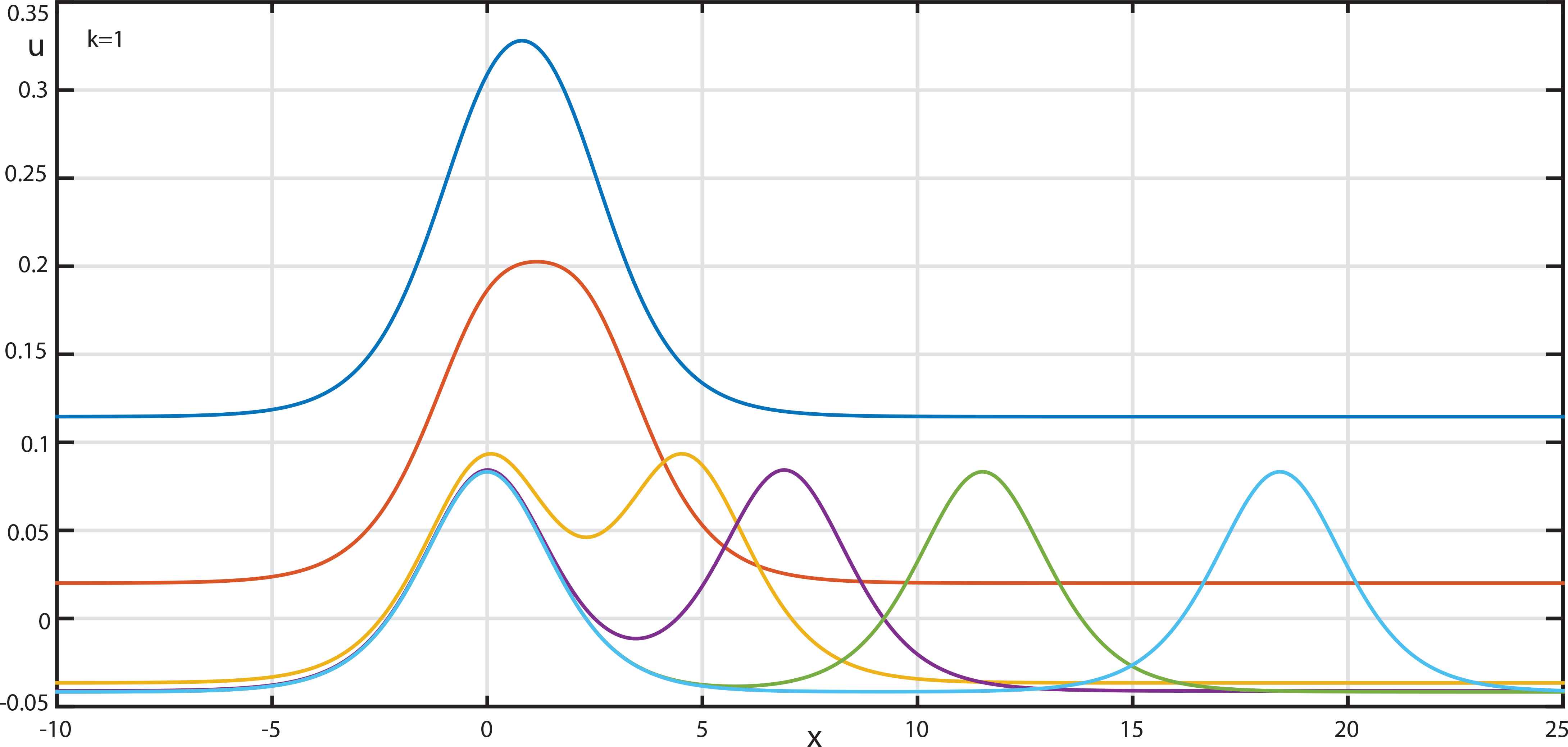
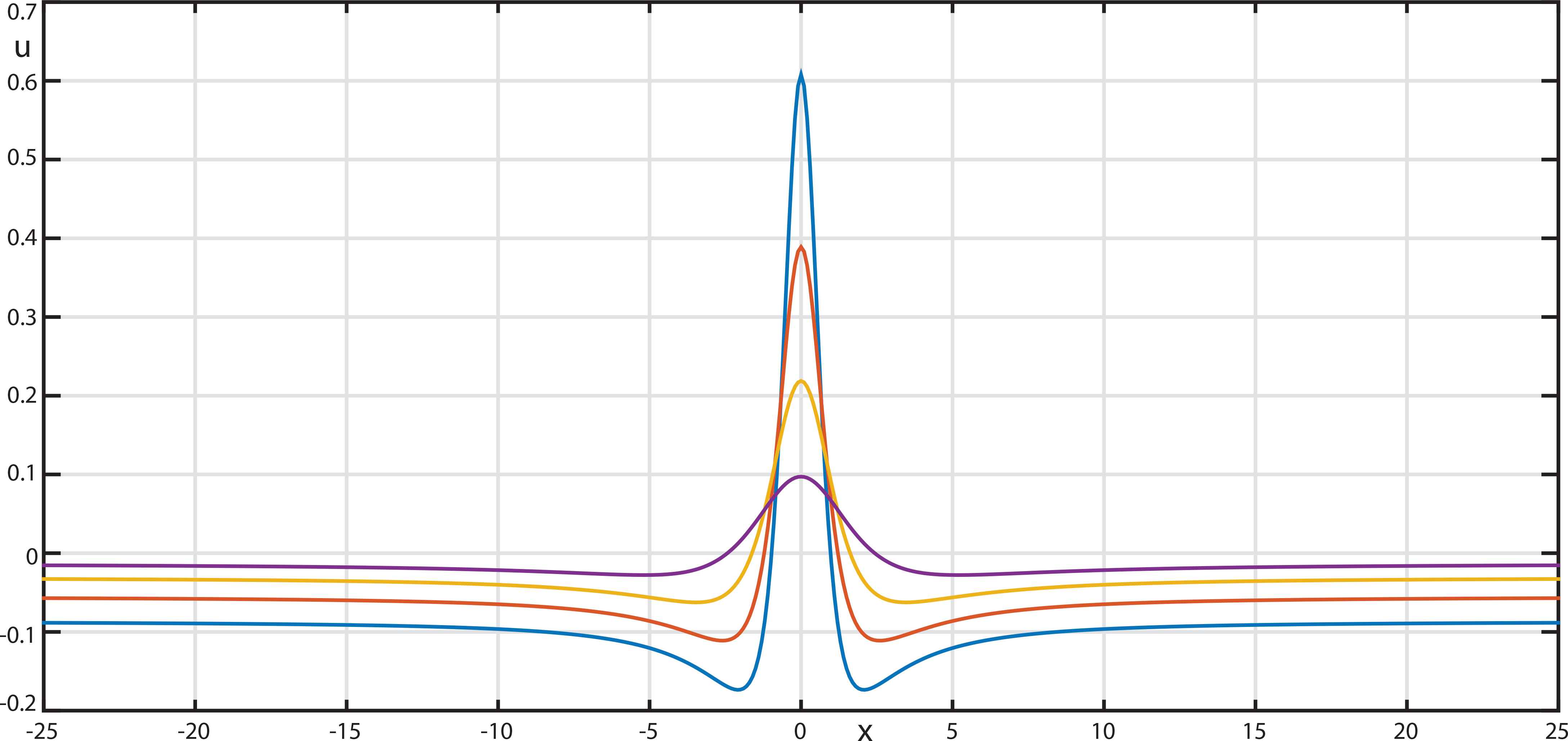
Figures 1–3 demonstrate the typical profiles of the solitons obtained. As can be seen, the exponential solitons of the first family (3.17) degenerate to the system of two noninteracting kinks (Figure 1). In other words, these solitons can be interpreted also as the strong bound kink states, not as the simple alone soliton. Figure 2 corresponds to the soliton family (3.18), while Figure 3 corresponds to the algebraic solitons (3.21)
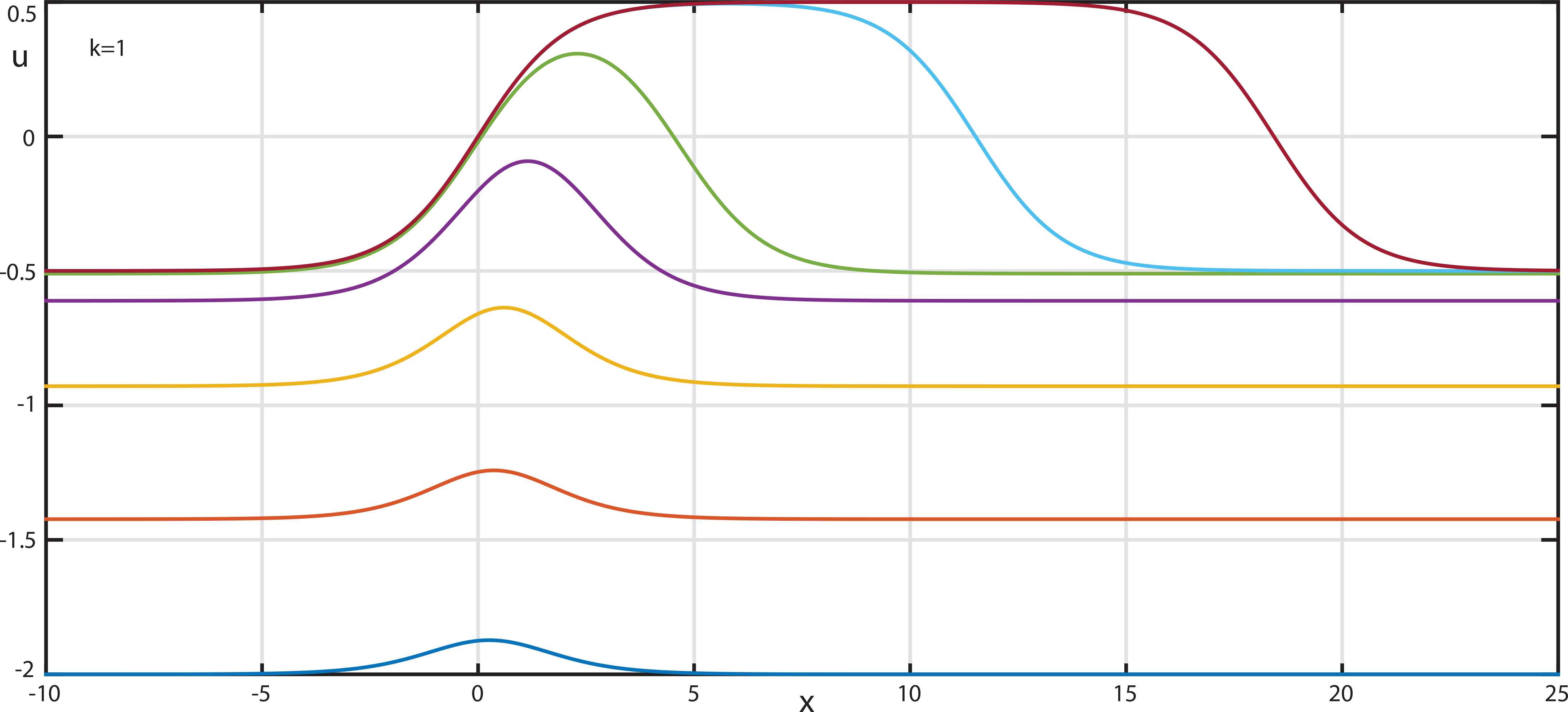
The typical profiles of the soliton family (3.17) of the MKdV − equation.
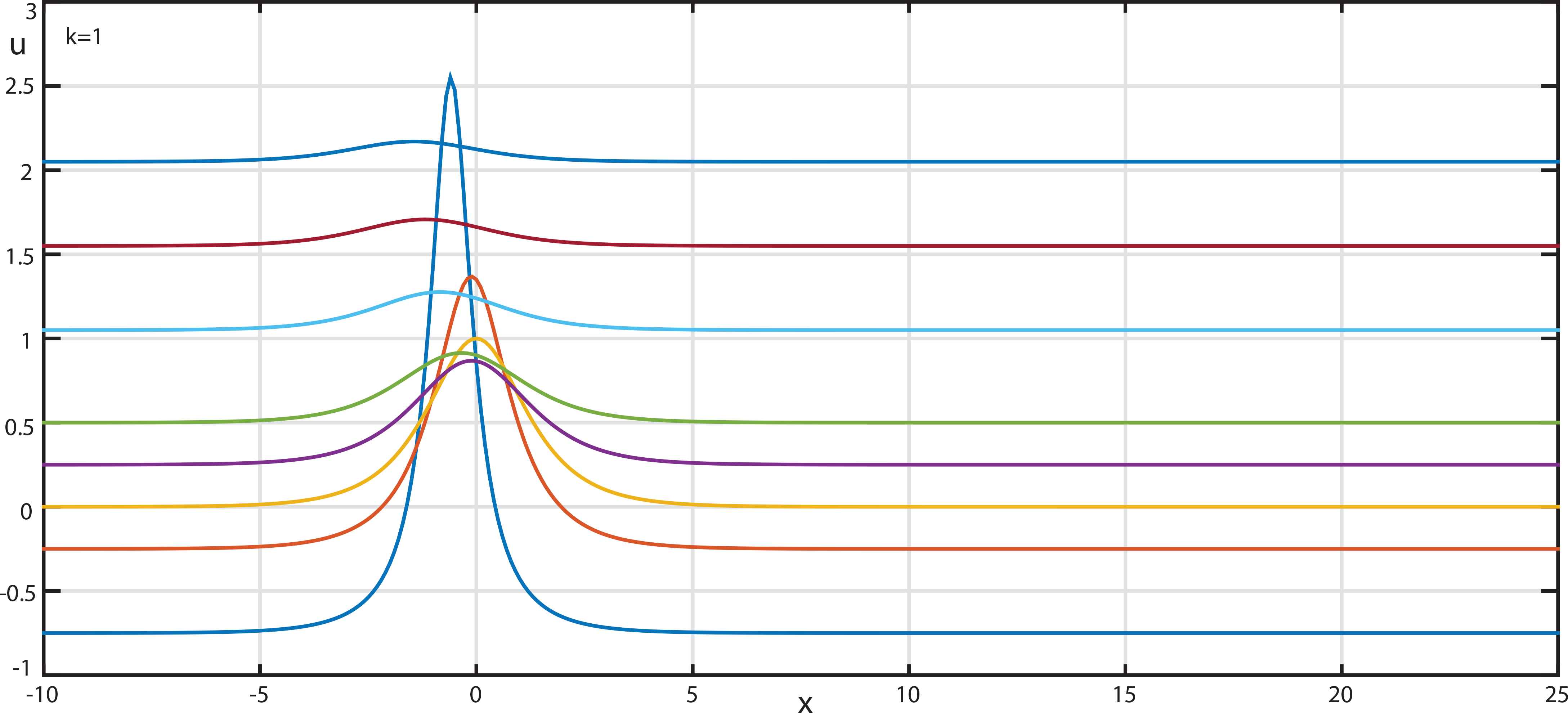
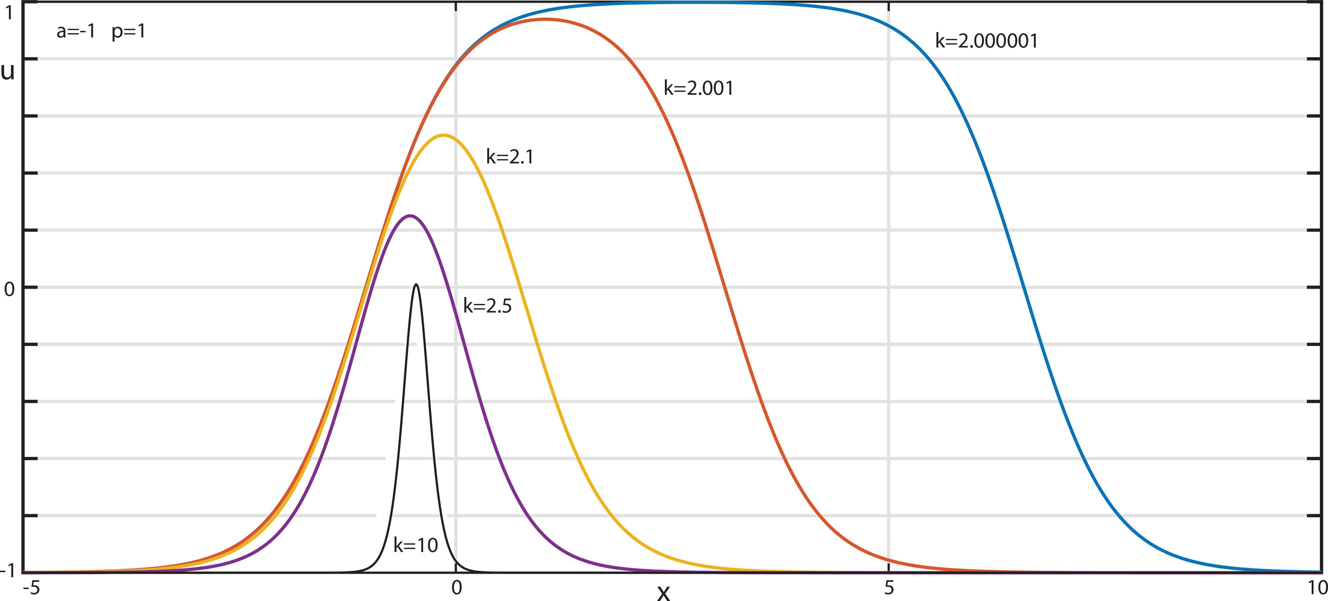
The typical profiles of the soliton family (3.18) of the MKdV + equation.

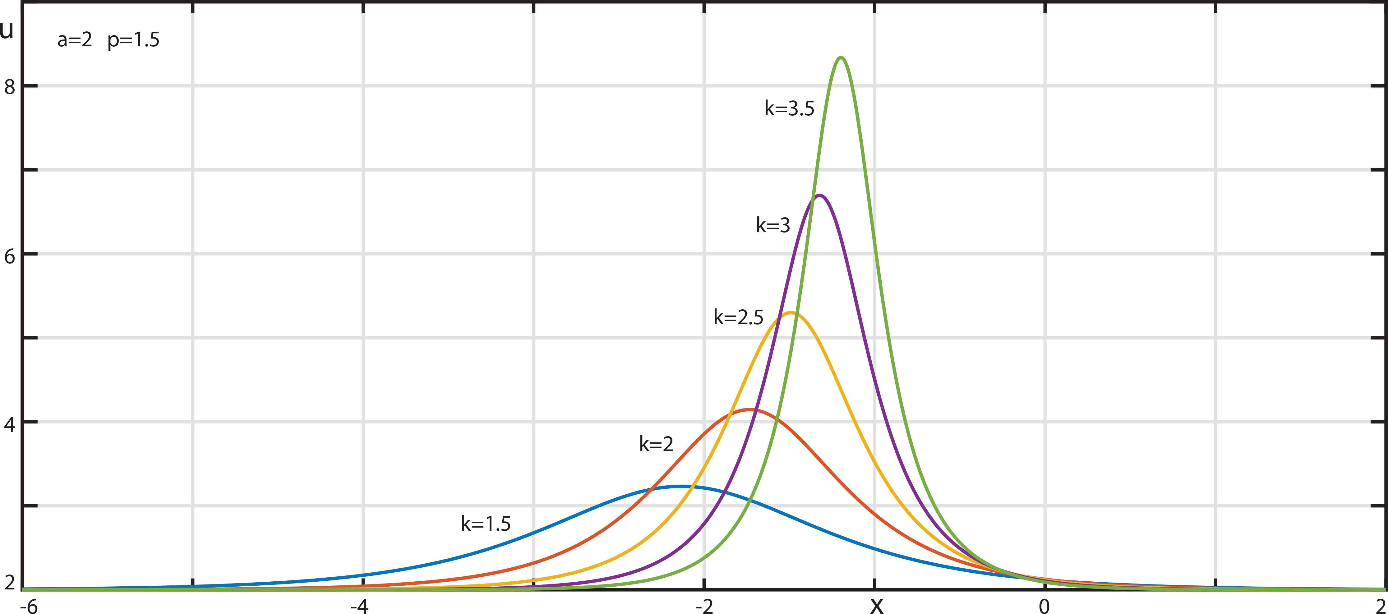
The typical profiles of the algebraic solitons (3.21) of the MKdV + equation.
The solutions (3.18) and (3.21) by themselves are known. They can be found, e.g., in the book [2]. While to our knowledge the strong bound state of the kinks (3.17) for the MKdV − has not attracted the attention of researches. Using the SFs found, two-soliton solutions of the various mixture types can be obtained. In particular, the solution describing the interaction between the kink (2.11) and the just mentioned two-kink strong bounded state (3.17) is as follows
The interaction is simple and without any resonance despite the very close wave numbers and duration, see Figure 4. In our opinion, at the present moment, obtaining of such two-solitons solutions in itself is not so interesting and important as the analysis of the SFs and general character of the interactions.

3.2. The KK equation
The KK equation has the following form
After that, starting from the remaining equations in (2.32)–(2.34), one arrives at the compatible systems consisting of Eqs. (2.25) for S1,2, Eqs. (2.28), (2.29) for α, β, γ together with the new equation for W0 specific namely for (3.23)
Besides, the following expressions for C1 and C2 take place
Just as in the case of the MKdV before, this system will give two evolution equations to the modulation functions θ1,2 with the only link between them
Now we need to obtain the expression for v and analyse what types of the solitons one deal with. To do this, for the usual exponential solitons one will recalibrate θ1 and θ2 in (3.29), (3.30) in the same manner (3.15) as previously for the MKdV. For d1,2 and v Eqs. (3.29), (3.30) at θ1, θ2 = 0, i.e. when only the soliton without a perturbation exists, give
The related expression for the soliton is
Here the real, nonsingular solution will be obviously if, first, s is real (i.e. s2 > 0 or a > −k2 / 6 and suitable d1,2, see (3.32)). But not only. If s is pure imaginary (s2 < 0. or a<−k2 / 6), then expression (3.33) can also be rewritten as
Figures 5–7 show the typical profiles of all the above soliton families, (3.33), (3.34) and (3.36). Again, (3.33) can be considered as the strong bound state of the simpler solitons. To the best of our knowledge the full and exhaustive researches of all three families and all the cases of these solitons (or the above soliton bound states) are not presented in the literature. Using the SFs, the interactions between the different families can in particular be investigated.
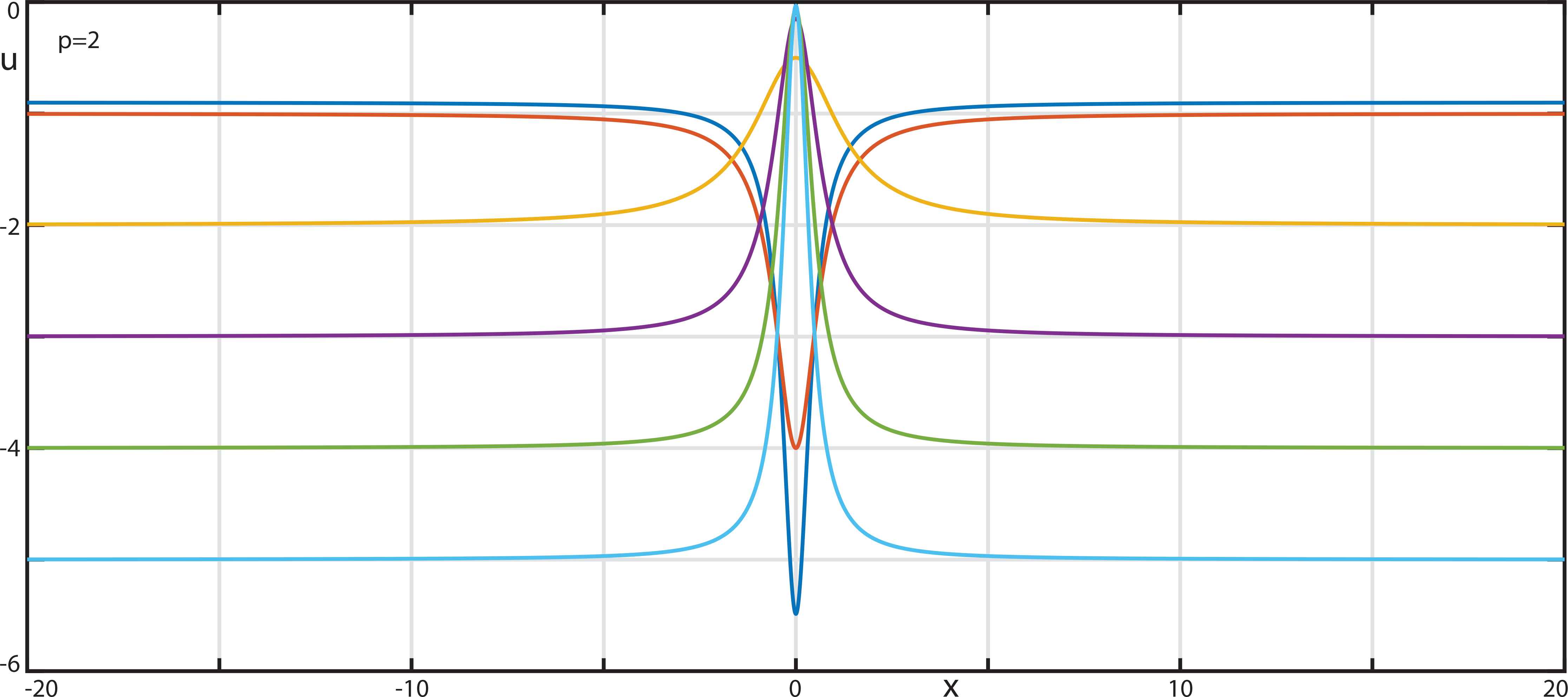
The typical profiles of the soliton family (3.33) of the KK equation.
The typical profiles of the soliton family (3.34) of the KK equation.
The typical profiles of the algebraic solitons (3.36) of the KK equation.
3.3. The A± equation
As was demonstrated in [8], the one of the powerful features of the MSP along with the transparency of the phenomenon of soliton interactions themselves is the possibility to find new nonlinear equations with a prescribed SF structure. The following equation
From the leading equations in (2.33), (2.34), one find that there are two opposite branches with W1,1 = 1 and W2,1 = −1, and the expansion (2.30) is of the form
The system of the remaining equations (2.32)–(2.34) is however not so simple. And not only because it is huge enough but also because it appears there are two dramatically deferent cases. As the one solution the following system in the involution takes place: the evolution equations (2.25) for S1 and S2 with
Basically, the last ones give the expressions for W0 and γ. In particular, excluding W0 from the former, we will obtain the expression for u(x, t) (3.38)
In other words, now it is possible to proceed to the equations and expressions with respect to the phase functions θ1 and θ1, because all available functions, namely S1,2, C1,2, α, β, γ are their expressions (see (2.35) with k1,2 = k and (2.37) or (2.36) and (2.38)). As a result, we will have only two evolution equations from (3.39) with the one constraint (3.43)
What soliton solutions do they associated with? Again, let us introduce the recalibration (3.15) and set θ1,2 = 0 to take away any perturbations. The system (3.44), (3.45) gives the expressions for the unknown d1,2 and the dispersion relations v = v(k)
After that the SF (3.42) gives the clear soliton solution
This solution is the analogue of the solution (3.17). For real a and suitable d1,2 in (3.47) this is the real, nonsingular soliton of the A +. But setting a → ia and u → iu, we will obtain real nonsingular soliton of the A −
For the algebraic soliton with the recalibration (3.19) in (2.36), Eqs. (3.44), (3.45) give
So, finally after the change a → ia and u → iu we have the real nonsingular algebraic soliton of the A −
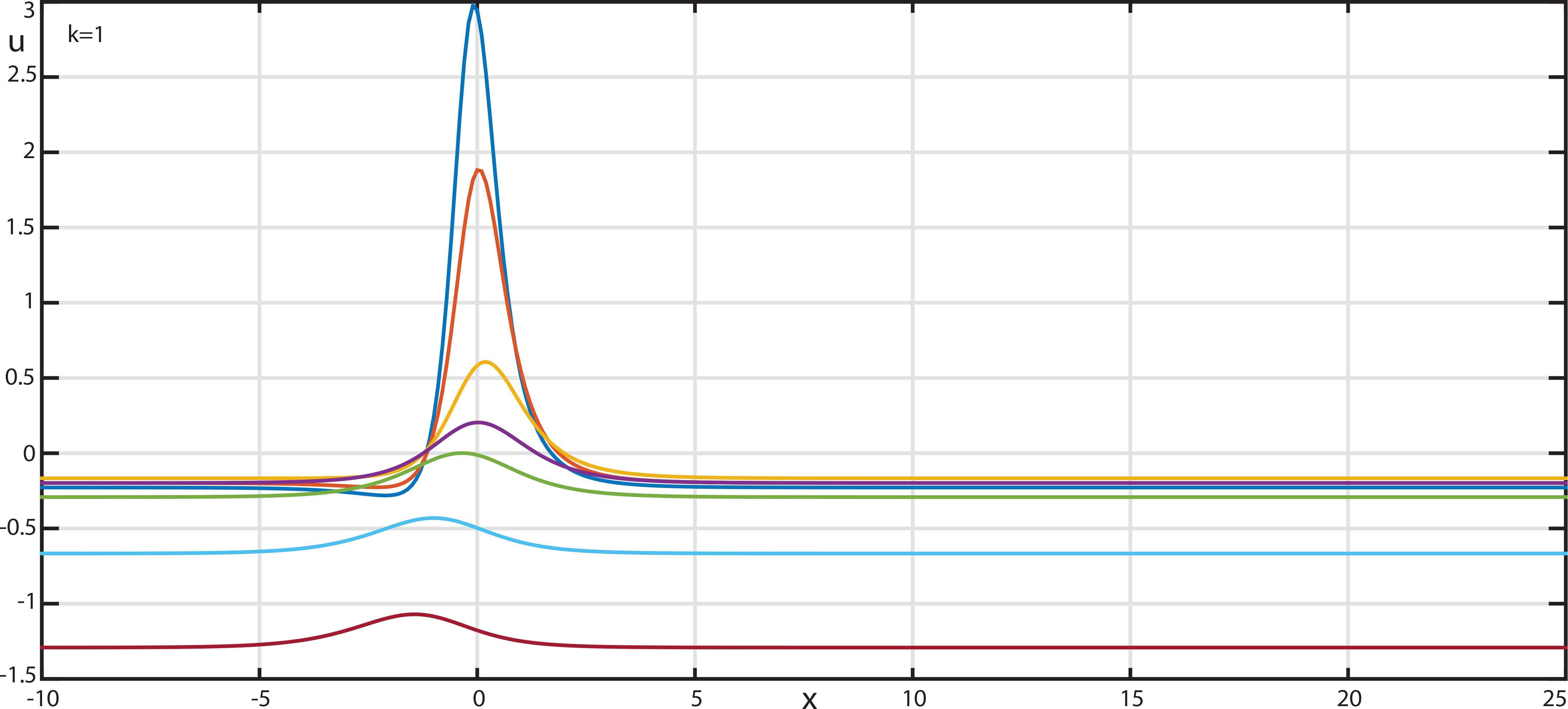
Figures 8–10 depicts the typical profiles of the above solitons.
The typical profiles of the soliton family (3.48) of the A + equation.
The typical profiles of the soliton family (3.49) of the A − equation.
The typical profiles of the algebraic solitons (3.50) of the A − equation.
Now recall that the system (2.32)–(2.34) with (3.38) for Eq. (3.37) has another solution different from (3.39)–(3.41). This second solution may seem paradoxical. It shows that if W0 = 0, α, β and γ can be arbitrary! This means that introduction of the link (2.26) between V1 and V2 is not essential. After substitution (3.38) into our Eq. (3.37) we can immediately equate the coefficients at the monoms
In terms of the phase functions θ1, θ2 (3.52) give two evolution equations and the one constraint
In contrast to the analogous expressions (3.44)–(3.46), all the expressions (3.53)–(3.55) do not depend on θ1, θ2 explicitly, so that they appear to be invariant with respect to the change θj(x, t) → θj(x, t) + Δj(j = 1,2). That is both kinks associated with V1, V2 in (3.51) can be positioned independently. Simultaneously, the SF says that they do not even interact with each other, their superposition is just linear. Any interactions take place only with the perturbation field. The related clear two-kink expression is
For the degenerate case with p = 0 (3.56), (3.57) is just two similar kinks moving with the identical velocities and identical asymptotics uk(∞, t) = 0. While for p ≠ 0 this is already the nonstationary structure. Its kinks have the different velocities |v1 − v2| = 8|p|, and its asymptotics are also different
The obtained results shows that for Eq. (3.37) together with the along kink solutions there exist both their strong bound states, the bell-shape solitons (3.48), and their absolutely noninteracting configurations (3.56) for the special choice of the wave numbers (3.57). And both complexes elastically interact with perturbations.
4. The Linearization and Parametrization of the SFs and the Soliton Interactions Analysis
The full SF analysis is not impossible and can gives interesting and important information [6]. However, as a rule, such SFs are huge enough. For our cases with two branches there is one more difficulty, the full SFs include two linked modulation functions. Fortunately, there are many characteristics of the soliton–perturbations interactions which can easily be obtained from the linearized SFs. Moreover, for the SFs generated by two branches there exists the simple procedure allowing one to introduce the only modulation function or to ‘parameterize’ such two functions SFs. This section is devoted to these procedures and to such analysis. Add here those linearized SFs are of their own rights as well. For instance, they can be applied also for describing week interactions [17], bounded soliton states [23,24], stability [21,22], etc. See in this connection also the works [25,26].
4.1. The MKdV equation
We will consider the formulae for the soliton family (3.17) of the MKdV − equation (3.1) first, and then these formulae will be extended to other cases, (3.18) and (3.21). One will begin with the linearization of Eqs. (3.10), (3.11) to the function θ1 and θ2 and introduce the small parameter ε for this in the following obvious manner
Remaining the terms up to the first order with respect to ε, one has
First, we can assume a ≠ 0 here, because this would lead to the singularity in the solutions (3.17). The special symmetrical structure of the constraint (4.3) allows one to turn easily to the only modulation function. Indeed, first of all notice that (4.3) is the inhomogeneous linear ordinary differential equation with respect to φ1 or φ2, and hence
Where φj,p are some particular solutions, while φj,p are the general solutions of the related ODEs D1φ1 = 0, D2φ2 = 0. Since (4.3) can always be converted to the identity
The situation with the related expression for u
Let us now consider how the linearization can be used for analysis of the interactions of the solitons with linear waves and with other solitons. The function φ with the asymptotics φ(± ∞, t) = φ± ∞ = const corresponds to usual elastic soliton–perturbation interactions [6]. While the states of the soliton before and after the interactions distinguish just by its phases with the shift depending on the difference φ + ∞ − φ−∞, the expressions for the perturbations in view of u1 in (4.6) with (2.39) are as follows
Such a transfer function can also be used to determine the phase shifts of other solitons after the interactions. Indeed, the phase shift of the whole soliton is obviously identical to the phase shift of its exponential fronts, say, the left front, e.g. for (3.17) one has
Here the constant term is inessential because is already included into u0 (4.6), just the second exponential one is needed. So, this transfer function gives the soliton phase shift dependence on the wave numbers of both solitons taking part in the colliding
As was demonstrated in the previous section, the real value exponential soliton (3.18) for the MKdV + is basically the imaginary version of the soliton (3.17) of the MKdV − and can be obtained from the latter via the simplest transformation a → ia, u → iu. For its perturbed version we should do the same also for the perturbation function, i.e. φ → iφ. So, we will have the parametrization
This case is more interesting than the previous one with the MKdV − solitons. In particular, here the functions φ1,2 appear to be also complex, see (4.8). As a result, T1 and T2 may oscillate even for not oscillating φ, see (2.51), (2.52) for the ingredients in u0 and u1 (4.9), here
All the above analysis of the SF is also suitable for this case in the whole volume.
Deriving all the above formulae, we assumed that a ≠ 0 in (4.3). What will we have when a = 0 however? First of all, in this case the MKdV − soliton (3.17) has the singularity on the real axis, so it is necessary to consider the case with the MKdV + (3.18). Let us return to Eqs. (4.2), (4.3). Now instead of (4.4) they will be
The second equation in (4.11) is very simple, and the parametrization with the new function φ(x, t) is of the form
So that for u0, u1 in (4.5) one has
In contrast to the analogous expression (4.9), here u1 in (4.13) contains the function φ itself. This means that for the small linear perturbations their interactions with the soliton do not result in the phase shift of the last one. Indeed, for the linear perturbation before and after the interaction one has from (4.13)
For localized perturbations up(∞, t) = 0 corresponding to asymptotics φ(± ∞, t) = φ± = const this immediately means φ± ∞ = 0, and as the consequence the absent of any soliton phase shift. Figure 11 corresponds to such an interaction, while Figure 12 to the interaction of the type considered previously (4.9). To be precise, both they depict the computer simulation for the MKdV + equation linearized on the soliton backgrounds v0 (3.18)
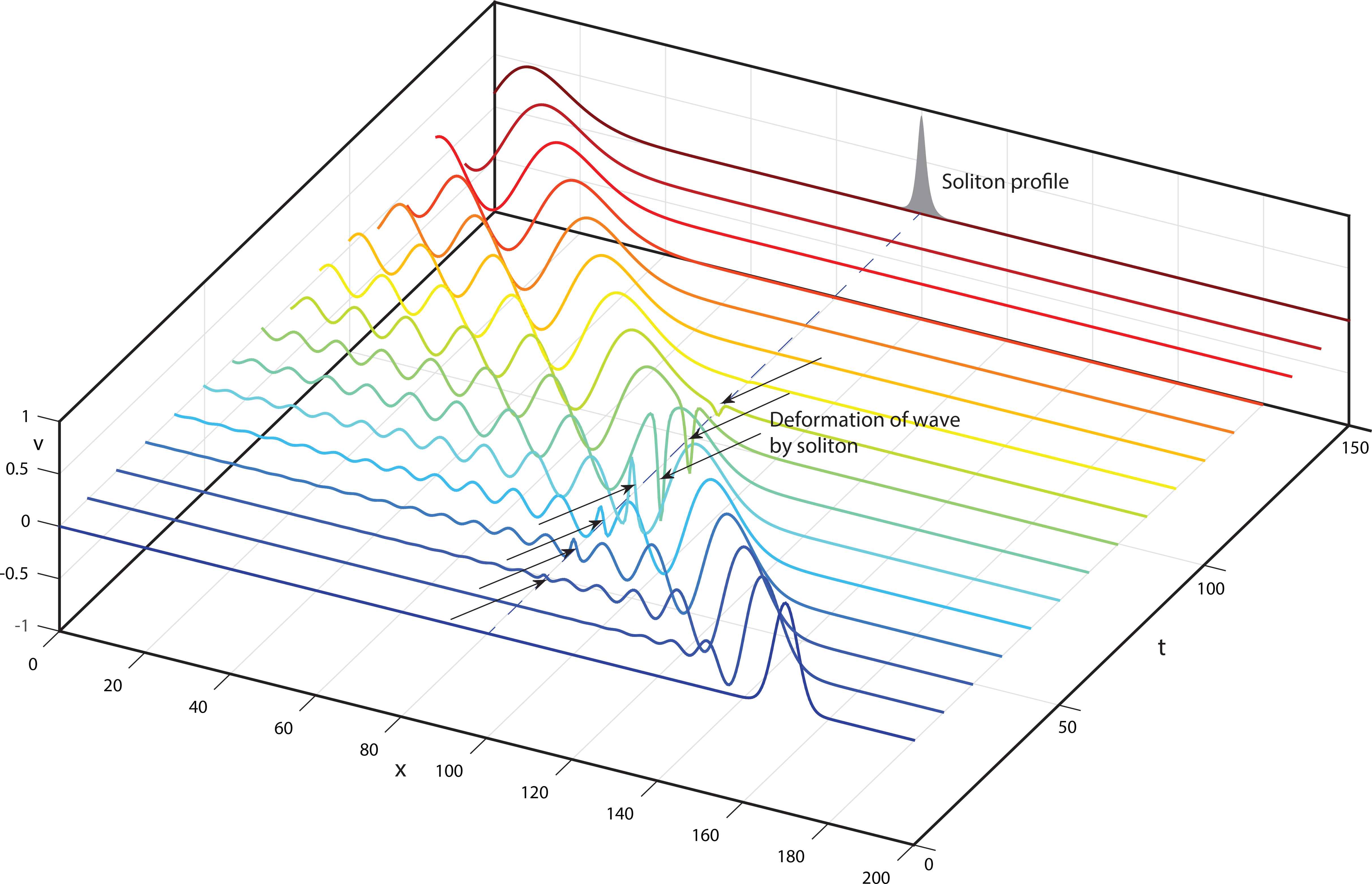
The computer simulation of the first order perturbation equation (4.15) corresponding to the interaction with the SF (4.5), (4.13) of the MKdV + soliton (3.18) (k = 1, a = 0) and some arbitrary linear wave package. The coordinate system is moving together with the soliton. The soliton phase shift is totally absent.
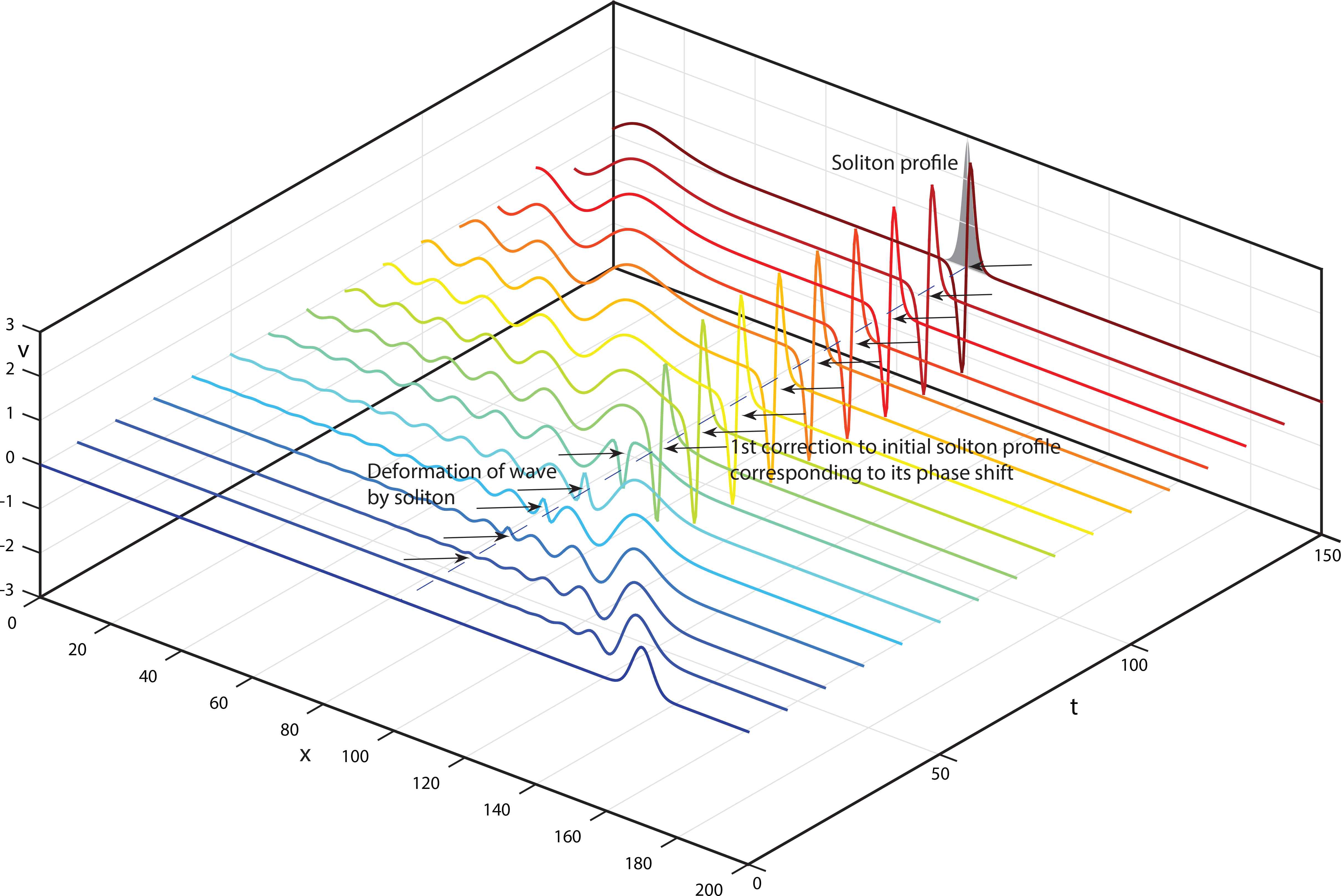
The computer simulation of the first order perturbation equation (4.15) corresponding to the interaction with the SF (4.5), (4.9) of the MKdV + soliton (3.18) for k = 1 and a = 0.5 and some arbitrary linear wave package. The coordinate system is moving together with the soliton. The powerful soliton phase shift takes place after the interaction.
Next, from (4.14) the transfer function is
In conclusion let us consider the case (3.12)–(3.14) corresponding to the algebraic soliton (3.21). It is the most simple one. Here the nonsingular solutions exist only for the MKdV + and a ≠ 0. In the view of the limiting relations (2.43)–(2.49) all the formulae sought can be trivially obtained from the analogous formulae (4.8)–(4.10). The parametrization (4.8) remain the same. While for the SF, from (4.9) one has
Both u0 and u1 are pure real in view of (2.51), (2.53), here
And because of the identical asymptotics of P1,2 (2.41) the expressions being obtaining from u1 (4.16) for the perturbation after and before the interaction are identical
So there is no effect of the soliton to it finally, the algebraic soliton is transparent. However, the soliton itself experiences the phase shift 2εa(φ + ∞ − φ− ∞), see (4.17), as usually.
4.2. The KK equation
As was said and demonstrated above, all the relations (3.29), (3.30) to θ1, θ2 and the SF (3.31) itself for the KK equation (3.23) are huge enough. So, we are obliged to confine ourselves in our narrative by only the main algebra and results. Fortunately, both the algebra and the ideas basically remains the same as for the MKdV.
Instead of the original equations (3.29), (3.30) to the modulation functions θ1 and θ2 in the SF (3.31) the linearization procedure with (4.1) θj(x, t) = εφj(x, t) + o(ε)(j = 1,2) gives two linear evolution equations
Then introducing into (4.18), (4.19) the parametrization with the new function φ(x, t)
Having in the hands the formulae (4.21), we can study the interactions features. The limited values of the functions T1,2 (2.39) are directly associated with the asymptotical states of the perturbations before and after the interaction (in the infinity in the left or in the right of the soliton). As a result, for the perturbation before and after the interaction the expression u1 in (4.21) gives
As a consequence, for the transfer function
The formulae (4.20)–(4.23) themselves are right both for the soliton (3.33) and for (3.34) without any changes. However, for the latter, the parameters s will be purer imaginary. The expressions for u0, u1 (4.21) will be real in any case (see (2.51), (2.52) for their ingredients), but φ1,2 in (4.20) appear to be complex. So, the SF will include sine and cosine functions. For μ1, μ2 we will have
For the nonsingular algebraic soliton (3.36) (a < 0) all analogous formulae can be obtained from the above formulae for the exponential solitons as the limit at k → 0 (see (2.48), (2.50)). Instead of (4.20), the following expressions take place, see (3.35),
While (4.21) gives
As well as the soliton (3.36) itself, u0, u1 (4.24) in the SF are real in view of (2.53). Also, the expressions
4.3. The A± equations
The algebra and formulaes of the linearization of the A± equations (3.37) principally remain the same as in the cases with the MKdV and KK equations. So, only their main points and final results are given here.
4.3.1. The bell−shape exponential and algebraic soliton cases
The transition to the linearized versions of the determining equations (3.44), (3.45) via the substitution (4.1) θj(x, t) = εφj(x, t) + o(ε)(j = 1,2) gives the pair of the linear evolution equations
Eqs. (4.25) allow the parametrization with the new function φ(x, t)
In terms of this new function the linearized SF will be of the form
The related expressions for small, linear perturbations from (4.27) are as follows
For the exponential soliton (3.49) of the A− equation it is enough to use the change a → ia and u → iu. Instead of the formulae (4.26) and (4.27), one will have
As seen from (4.29), φ1,2 are complex here, so it is needed to take into account the relations (2.51) and (2.52) with
The expressions for up± ∞ and
As the comment note that at a4 − p2 = 0 for the SFs (4.27), (4.30), (4.31) of all three soliton families there take place their degeneration. Indeed, in this case all formulae (4.26), (4.27) and (4.29), (4.30), (4.31) stop to depend on φ explicitly, only its derivatives remain. First, this means that in this case there are only three modulation parameters {φx, φxx, φxxx} instead fore. Second, we here have the same situation as with the MKdV degeneration (4.12), (4.13) (it is possibly to pass to another function φx → φ in the above formulae for the clearness), when any soliton phase shift after the interactions is absent. This effect takes place for both exponential soliton families (3.48) and (3.49), in contrast to the MKdV case with the family (3.18) only.
4.3.2. The configuration from the two noninteracting kinks
From the viewpoint of the formulae the case of the noninteracting kinks (3.56) in contrast to the alone bell-shaped soliton case has the only deference, namely the additional arbitrary constant Δ1,2 in the kink phases (3.56), that makes them independent on each other. The system of the linearized determining equations (3.53) after the change θ1,2 → Δ1,2 + εφ1,2 + o(ε), are fully similar and is
After the parametrization of (4.32) in view of (4.33) with the function φ(x, t)
Notice that the transfer function from (4.35) for these two-kink configuration
5. Conclusion
The paper develops further the general theory of solitons and soliton interactions proposed by the author [3]– [11]. Theoretically, the article generalises the direct technique for constructing SFs [10]. And as its applications, the SFs for the MKdV, KK and A ∓ equations are considered. The results have been obtained for them concern both the fuller and deeper description of the known soliton solutions and the principally new results concerning their superposition properties and their interactions with other waves. The main points can be formulated in the following manner:
- 1.
The above technique is generalized to the case of multibranches with constraints.
- 2.
The formulae for the limit passage from the SFs for exponential solitons to algebraic ones are introduced.
- 3.
The proposed generalization is used to derive the SFs for the solitons of the MKdV, KK and A ∓ nonlinear PDEs in the cases when one branch technique does not work.
- 4.
For all three equations the SFs for the bell-shape exponential and algebraic solitons are derived. It is shown these solitons can be considered as the strong bound states of two identical kinks (MKdV, A ±) or two simpler bell-shape solitons (KK). For the A ± the two noninteracting kinks configuration is also found and studied.
- 5.
Aside from the full SFs, their much more simple linearized versions are also investigated, and the parametrization procedure is introduced into the approach.
- 6.
The linearized SFs are used for investigation of some interaction properties of the above solitons.
- 7.
Based on the structure of the SFs constructed, the possible difference in the interactions (smooth and oscillating character) are indicated for the various SFs.
- 8.
Based on the form of the SFs, the degenerated cases (i.e. with no soliton phase shift) are indicated for the MKdV and A ∓ and confirmed by the computer simulation.
- 9.
On the example with the KK equation solitons the common viewpoint about the uselessness of the use of identical branches is disproved.
Acknowledgements
The author is grateful to Professor T Wolf for his assistance and together with Computer Canada and SHARCNET for the afforded computer facilities.
References
Cite this article
TY  - JOUR
AU  - Alexander A. Alexeyev
PY  - 2021
DA  - 2021/01/06
TI  - A Multidimensional Superposition Principle: Classical Solitons IV
JO  - Journal of Nonlinear Mathematical Physics
SP  - 1
EP  - 33
VL  - 25
IS  - 1
SN  - 1776-0852
UR  - https://doi.org/10.1080/14029251.2018.1440740
DO  - 10.1080/14029251.2018.1440740
ID  - Alexeyev2021
ER  -