Decomposition of 2-Soliton Solutions for the Good Boussinesq Equations
Authors
Vesselin Vatchev
School of Mathematical and Statistical Sciences, University of Texas Rio Grande Valley, One West Boulevard Brownsville, TX 78520, US,vesselin.vatchev@utrgv.edu
Received 12 November 2019, Accepted 28 January 2020, Available Online 4 September 2020.
We consider decompositions of two-soliton solutions for the good Boussinesq equation obtained by the Hirota method and the Wronskian technique. The explicit forms of the components are used to study the dynamics of 2-soliton solutions. An interpretation in the context of eigenvalue problems arising from KdV type equations and transport equations is considered. Numerical examples are included.
The N-soliton solutions of nonlinear PDE describing shallow water waves (SWW) as the Kortewegde Vries (KdV), the KP hierarchy, Boussinesq and more recent Camassa-Holm (CH), Depasperies-Procesi (DP) and other PDE have been subject of numerous recent studies. The interest stems from the mathematical and the physical importance of those solutions. Explicit forms of the N-soliton solutions also can provide better modeling of SWW. There are well developed analytical methods for obtaining explicit solutions via recursion operators, Hirota bi-linear method or the Wronskian technique but the physical interpretation is obscured by the complexity of the formulas. A few papers on interpretations and discussion of possible decomposition are [2], [13], [21], [5].
The intend in this work is to study the properties of 2-soliton solutions for one of the simplest and oldest models, the Boussinesq equation. The general form of the Boussinesq equation is
utt+a1uxx+a2(u2)xx+a3uxxxx=0,
where ai, i = 1, 2, 3 are real numbers and a2a3 ≠ 0. In the case a3 > 0 it is known as the ‘good’ Boussinesq equation and is equivalent to
vtt+(v2)xx+vxxxx=0,
under the transformation
u(x,t)=−a12a2+a3a2v(x,a3t).
We consider the ‘good’ Boussinesq (gB) equation as defined in [6]
utt−uxx+(u2)xx+13uxxxx=0.(1.1)
The equations has a well known Lax pair
φxxx+vφx+wφ=λφ,φt=−φxx−vφ.
PDE with a Lax pair is usually a definition of integrable system, [11], and can be solved by the inverses scattering transform (IST) introduced by Clifford, Greene, Kruskal, and Muira, [9]. By utilizing IST Ablowitz and Segur, [1] provide an almost linearization of the KdV
ut−6uux+uxxx=0(1.2)
with respect to the spatial variable in terms of an eigenvalue problem with the Lax pair
φxx=(λ−u)φ,φt=−4φxxx−3uxφ−6uφx.
Many of the SWW equations posses a single traveling wave of the form sechr(ax − bt) for r = 1, 2 and a, b independent of x. The duality of a wave and a particle of the one soliton solution is often considered, [5]. The results presented in this work are also interpreted in a direction of that comparison for the case of two-soliton solutions. In order to clarify this we present a brief discussion on the duality of one soliton solution in the context of KdV and gB.
A one soliton solution to (1.2) for p > 0 is k(x, t) = psech2p(x − 4p2t − w), where w is a real phase shift. On the other hand a one soliton solution to (1.1) is not defined for all p but for a range of p that can be represented by two of the solutions, m1, m2 of the cubic equation μ3−34μ=λ, |λj|⩽14 and p=12(m1−m2). Let M=m1+m22 then soliton solution to (1.1) corresponding to such p is the function b(x, t) = psech2p(x − 2Mt), [6]. The time coefficients in the phases of the two ‘sech’ functions are different and we can not compare k and b for any time t and any x. We will compare k and b at any fixed time t = t0 with a phase shift for KdV w(t0) = (4p2 − M)t0, and hence v(x, t0) = k(x − w/p, t0).
The two equations describe traveling waves that in turn represent an energy transport. The function ψ(x, t) = sech p(x − 4p2t − w) is a solution of the time independent equation from the Lax pair for KdV ψxx = (p2 − k)ψ with potential k = pψ2. The function Φ(x, t) = sech p(x − Mt) is a solution of the transport equation
Φt+MΦx=0,
and b = pΦ2. The equation for ψ is an eigenstate equation. The function φ(x,t)=(em1x−m12t+em2x−m22t)−1b is a solution of the wave equation ϕt = ϕxx + bϕ. Since k(x − w(t0)/p, t0) = b(x, t0) for any t0 we can consider the function ψ defines the steady state of a ‘particle’, and k = pψ2 can be considered as a weighted energy distribution and potential. The function ϕ is a solution of the real time-dependent Schrodinger equation corresponding to the energy state ψ(x, t0) so e−(m1+m2)x−(m12+m22)tb could describe the probability distribution of the particle in motion. On the other hand the energy is confined into the soliton and the transport equation governs the transfer of energy which is constant in time. Comparing the solutions of KdV and gB is justified by the fact that both are approximations of the same order, [18], of the Euler’s equation in Fluid Mechanics.
In the next section we include brief overview of decomposing N-soliton solution into components with an emphasis on KdV type equations.
Section 3 contains decomposition of 2-soliton solutions of gB with components that satisfy similar differential equations as in the case of a single soliton. In sections 4, 5 we compare the resulting solutions to provide interpretation in the context of the discussion for one soliton, including numerical examples. The last section is a discussion of the results presented and further directions.
2. Decomposition for 2-Soliton Solutions
A general natural way method for decomposing a N-soliton solution uN onto N interacting components (interacting solitons)
uN=∑k=1N(uN)k
seems to be by a recursion operator Φ(u) and a corresponding hierarchy, [8], [4],
ut=Φm(u)ux=Km(u),m∈N.
In this case for real ckm the spatial derivative of uN = uN(ξ1,...,ξN), ξk=x−ckmt+qk is
(uN)x=∑k=1Nckmwk,wk=∂uN∂qk.
The operators Φ and K′m are a Lax pair
Φ(uN)wk=ckwk,(wk)t=Km′[wk]
and the N-soliton solution decomposes as follows
uN=∑k=1Nckm(uN)k=∑ckm∂x−1wk=∑ckm∂x−1∂uN∂qk,
which can be immediately calculated from the Hirota (or Wronskian) formula. The method of recursion operators has been used in many works, [4], [3], [7], [8], [15], to produce N-soliton decomposition for Burgers, KdV, mKdV, sine-Gordon, cubic Schrodinger and other nonlinear PDE’s. For the Boussinesq equation a recursion operator is presented in [20] but no decomposition of N-soliton solution discussed.
The Lax pair (Φ, K′m) is often not the ‘standard’ Lax pair related to the linear problem
Lψ=λψ,ψt=Amψ
and in general the eigenfunctions ψk and wk as well as the eigenvalues λk and ck are interrelated. For the KdV for example
wk=(ψk2)x,ck=λk=pk2.
Our interest is in nonlinear PDE modeling SWW. These equations usually are either directly derived from or related to the Fluid Eulers’ Equation. The simplest model equations are KdV and Boussinesq equations. They model unidirectional solitons and posses explicit and relatively simple N-soliton solutions. Models of higher order of approximation to the Euler’s equations and multi-soliton solutions are Camassa-Holm (CH), [23], Depasperis-Procesi (DP), [17], Novikov (N), [17], and Sawada-Kotera (SK), [22]. Recursion operators for some of those equation are known but with no simple analytical descriptions.
One of the goals in this work is to investigate decomposition of 2-soliton solution onto components related to lower order linear PDE. We consider known solution and the lower order equation from a Lax pair. For KdV this is the second order eigenproblem but for the Boussinesq L is a third order and we consider the second order wave equation corresponding to Am.
The Hirota method, with Wronskian solutions, Darboux and Backlund transformations are more often used to model 2-soliton solutions and their interactions in the setting of SWW PDE. For some of them fully explicit 2-soliton solutions are not known. For example, in [23] a 2-soliton solution for Negative order KdV is transformed to express the 2-soliton solution for CH. The 2-soliton solutions for the other shallow water waves present the same difficulty due to the complexity of the functions describing them. All of the equations posses a single soliton solution in sech(ax − bt) form but the construction of the 2-soliton solutions from two seed solutions is more involved. A common element in the most of the constructions is the Wronskian determinant
The most popular model for SWW is still the Boussinesq eqaution due to its simplicity but even in this case there are difficulties in considering 2-soliton solutions. In [17] a merging of two solitons, fusion, was reported. This is likely due to the fact that the Lax pair for gB has a third order spatial equation. Explicit N-soliton solutions for KdV and gB with elastic interaction, i.e. after the interaction only phase shifts occur, can be obtained by Hirota’s method, [10] and Wronskian determinants, [12], [6].
For the ‘good’ Boussinesq equation f and g are of the form
where m1, m2 are two solutions to the equation μ3−34μ=λj, |λj|⩽14 and ε = −1 corresponds to waves traveling in the same direction while ε = 1 corresponds to waves traveling in opposite directions.
Next by using the Wronskian technique and Hirota’s log substitution one can get 2-soliton solutions of KdV and gB equations in the form,
w=2(lnW)xx=2∂∂x(WxW).
We introduce the notations ci(x, t) = cosh(pix − Ti(t)), si(x, t) = sinh(pix − Ti(t)), and ti=sici for i = 1, 2. The x derivatives of ci, si are ci,x = pisi, si,x = pici, and |ti| < 1. We also define the KdV type Wronskian determinants
In the case of unidirectional solitons p2 > p1 > 0 and hence K > 0. The next result is an extension of results from [2] for characterization of k = 2(lnK)xx.
Lemma 2.1.
Ifψ1=s2Kandψ2=c1Kthen
k=2(lnK)xx=2p12(p22−p12)ψ12+2p22(p22−p12)ψ22
and ψiare solutions of the eigenvalue problem ψxx = (λ2
− k)ψ for the eigenvalues p1and p2correspondingly.
Proof.
By the Hirota’s substitution with Kx=(p22−p12)c1s2 and Kxx=(p22−p12)(p1s1s2+p2c1c2) we calculate directly that
and the result for ψ1 follows. Similarly, ψ2 is an eigenfunction corresponding to p2.
For Ti(t)=4pi3t we obtain the 2-soliton solution for KdV and the decomposition agrees with the one associated to IST, [9]. The result in lemma 2.1 holds for all functions Ti and we consider the potential function k as a weighted energy distribution of particles in the two states ψi with no interactions. There is no immediate PDE that can be associated to k for any choice of Ti and we will refer to k as KdV type potential. Ant advantage of the KdV type potentials is that they are well defined for solitons traveling in opposite directions.
3. 2-Soliton solutions for the ‘good’ Boussinesq Equation
In this section we derive decomposition of the 2-soliton solution for gB. The Wronskian determinant V=|fgfxgx| where f and g were defined in (2.1), generates a 2-soliton solution 2b = (lnV)xx for gB. The functions f and g are solutions of the following ODEs
fxx−(m1+m2)fx+m1m2f=0,gxx−(n1+n2)gx+n1n2g=0,(3.1)
with characteristic polynomials P1(λ) = (λ − m1)(λ − m2) and P2(λ) = (λ − n1)(λ − n2). Let θ1(x,t)=−(m1+m2)x2+(m12+m22)t2, θ2(x,t)=−(n1+n2)x2+(n12+n22)t2, D = n1 + n2 − m1 − m2, and L = m1m2 − n1n2.
Theorem 3.1.
For functions f and g, defined in(2.1), a two soliton solution b = 2(lnV)xxfor the gB has the following representation
The functions Φi= e−θiϕiare solutions of the transport-eigenvalue problem Φt + 2RΦx = Φxx + (−λ2+ v) Φ with R = M and λ = p1for Φ1, andR=n1+n22and λ = p2for Φ2and
b=8p12(Dgxg+L)Φ12−8ɛp22(Dfxf+L)Φ22.(3.4)
Proof.
To compute (lnV)x we use a column-wise differentiation of determinants
The last identity can be verified by using the Sylvester’s method to expand W(f, fx, g) along the second and third rows and first and second columns.
Since f and fx satisfy (3.1), multiplying the first row by m1m2 and the second by −(m1 + m2) and adding them to the last we get that
W(f,fx,g)=|ffxgfxfxxgx00gxx−(m1+m2)gx+m1m2g|.
Since, |ffxfxfxx|=(m1−m2)2e−2θ1=4p12e−2θ1 and gxx − (m1 + m2)gx + m1m2g = (n1 + n2 − m1 − m2)gx + (m1m2 − n1n2)g = Dgx + Lg then we obtain the the representation for 2ν1,x. For the second term the determinant |ggxgxgxx|=ɛ(n1−n2)2e−2θ2=4ɛp22e−2θ2 and fxx − (n1 + n2) fx + n1n2f = −(n1 + n2 − m1 − m2) fx − (m1m2 − n1n2) f = −(Dfx + Lf) and thus (3.2) follows.
Next we show that the functions φ1=gV and φ2=fV are solutions of the wave equation. From v=2VVxx−(Vx)2V2 and Vx = fgxx − fxxg it follows that
we get the identity for ϕ1. Similarly we can obtain the result for ϕ2 and (3.3).
By using the relation ϕi = eθiΦi and substituting in the wave equation we see that Φi are solutions to the corresponding transport-eigenvalue problems and b solves (3.4).
The decomposition for b holds in the case of solitons traveling in the same or opposite directions. The function g has a zero in the case of opposite directions but Φ22 has a double zero at the same location.
The two components of k from lemma 2.1 could be considered as two energy states of the eigenvalue problem with potential k, the steady state, ψ2 (has no zeros) and the excited state, ψ1 (has one simple zero). For gB we obtained two representations, (3.3) with components being solutions either to the wave equation with a potential b but with damping factors e−2θi or in case of (3.4) the transport-eigenvalue problem, with potential b. Next we compare the potential functions k and b and the corresponding components for the 2-soliton solutions corresponding to gB and KdV type potentials. For t → ±∞ both Φi and ψi, up to a constant shift approach sechi2. This can be interpreted as two ‘particles’ being in a time-varying steady state. At the moment of interaction one remains in a steady state, ψ2, while the other transition into an excited state, ψ1.
Let u=14log|(n1−m2)(n2−m2)(n2−m1)(n1−m1)|, v=14log|(n2−m1)(n2−m2)(n1−m1)(n1−m2)| and define s1*(x,t)=s1(x−u/p1,t), s2*(x,t)=s2(x−v/p2,t). Let P1i = P1(ni) and P2i = P2(mi), i = 1, 2. Then we have the following
Theorem 3.2.
Letσ=P11P12, b2=p222(|P22|−|P21|)2and in case of solitons, ε = 1, b1=b1c=p122(P12−P11)2and in case of chasing solitons traveling in opposite directions, ε = −1, b1=b1o=−p122(P12+P11)2then
b=2σp12(s2*B)2+2σp22(c1*B)2+(b2−b1)1B2.(3.5)
Proof.
First we notice that in the Hirota substitution the solution for gB can be generated by using the following determinant
Since D = n1 + n2 − m1 − m2 and L = m1m2 − n1n2 the identities 2Dp1 = −P22 − P21 and 2(DM + L) = P22 − P21 hold. The second term of b, in (3.1), in both cases is
To evaluate the first term of (3.1) we consider separately the cases for ε. For ε = −1 we have g=en1x−n12t−en2x−n22t=2e−θ2sinhp2(x−Nt)=2eθ2s2 with x derivative gx=n1en1x−n12t−n2en2x−n22t=2e−θ2(p2c2+Ns2) and similarly to the case for f the first term of b in (3.1) is
In the case of solitons traveling in opposite directions ε = 1 and g=en1x−n12t+en2x−n22t=2e−θ2coshp2(x−Nt)=2e−θ2s2 with x derivative gx=n1en1x−n12t+n2en2x−n22t=2e−θ2(p2s2+Nc2). In the same fashion as for f we have that the first term of b in (3.1) is
By adding up the last two identities we get the formula in case of chasing solitons. The derivation for solitons traveling in opposite directions is similar.
Next we show that the 2-soliton solution for gB obtained in theorem 3.1 is always positive.
Lemma 3.1.
For any x and t the 2-soliton solution b is positive.
Proof.
In the case of colliding solitons the coefficients b1 and b2 are always positive so we need to consider only the case of chasing solitons. In this case n1 < m1 < m2 < n2 and hence P11, P12 are positive while P21, P22 are negative. Since c1*⩾1 we have that
Furthermore since p2 > |p1| and σ > 0 we need to show that −p122(P11+P12)+p222(−P21−P22) is positive. The m’s and n’s are solution of the equation μ3−34μ=λj, |λj|<14 which roots can be expressed in trigonometric form for 0<α=13arccos(4λj)⩽π3
m1=cos(α),m2=cos(α+4π3),m3=cos(α+2π3).(3.6)
Thus −1⩽m3⩽−12. For α<β⩽π3 we have n1 = cos(β) > m1 and n2 is either cos(β+2π3) or cos(β+4π3). Let assume first that n2=cos(β+4π3), n3=cos(β+2π3) then from Vieta’s formulas we get that
where U(ξ)=2m32+3m2ξ+2ξ2−1. The linear function U′(ξ) = 4ξ + 3m3 is negative for any x < m2. Indeed, U′(ξ)⩽U′(m2)=4cos(α+4π3)+3cos(α+2π3)=3cosα2(tanα−73)<0 since 0⩽α⩽π3. On the other hand from the Vieta’s formulas it follows that U(m2)=m12−14⩾0, and hence U(ξ) > 0 for any ξ < m2. Both of the choices for n3, cos(β+4π3) and cos(β+2π3) are less than m2 the statement in the lemma is established.
In the next section we obtain necessary condition on the distribution of m’s and n’s such that the determinant B is nonzero. We also the properties of 1B2.
4. Analysis of the parameters of the 2-Soliton Solution for gB
In order to have non-singular solutions it is necessary to require that the Wronskian determinant B(x, t) > 0 for any real x and t. Initially, we consider separately the cases for ε, starting with chasing solitons i.e. ε = −1,
is a bi-linear function in t1, t2. Since t1 and t2 are hyperbolic tangents in terms of x and t it is clear that the values of the pair (t1, t2) are in the square with vertices
E={(−1,−1),(−1,1),(1,−1),(1,1)}
in the t1, t2 plane. The bi-linear function Tc attains its maximum and minimum at the elements of E. Considering the values at the vertices we obtain sufficient conditions for the distributions of the n’s and m’s. Direct computations lead to
then all of the values are positive and since c1, c2 are always positive we get that B is positive for any x, t.
The results from the previous section suggest that b is closely related to the KdV type potentials k, they both are expressed in terms of c1, c2. Similarly to the case of one soliton from the introduction we consider the spatial shifts u, v defined in theorem 3.2 in the two seed solitons,
Since p1=m1−m22, p2=n1−n22 in the case of chasing solitons, (4.1), we have p2 > p1 > 0 and hence T is positive for any choice of the parameters u and v. In the case of solitons traveling in opposite directions, (4.2), p1 < 0 and a necessary condition all values to be positive is p2 > |p1|. In what follows we assume that indeed p2 > |p1|.
Next we show that B and K are equivalent in the sense that there exist positive real constants a1, a2 such that a1K ⩽ B ⩽ a2K for any x and t. In such a case we write B ≈ K.
then0<θm⩽BK⩽ΘM<∞, or B ≈ K, where θm = min(η1, η2) and ΘM = max(η1, η2).
Proof.
In the case of chasing solitons the positive bi-linear functions Tc and T attain their extreme values at the elements of E={(ei,ej)i,j=12} and from BK=TcT we get that
0<minETcmaxET⩽BK=Tc(x,t)T(x,t)⩽maxETbminET<∞.
Direct substitution of u, v show that the ratio TbT has only η1 and η2 as possible values at E and this determins the choice for θm and ΘM. In the case of solitons traveling in opposite direction we notice that To(ei, ej) = Tc(ei, ej), i, j = 1, 2 and hence we arrive at the same estimate.
The explicit expressions obtained so far suggest that the main difference between b and k*
is in the ‘interaction’ 1B2. Next we show that the functions I=1B2 and J=1K2 indeed exhibit properties of interaction terms.
Lemma 4.2.
For the choices of the parameters as intheorem 3.2, I and J are bell-shaped,limx→+∞I(x,t)=0,limx→+∞J(x,t)=0, with a single maximum tending to zero as t → ±∞, and1K=W(ψ1,ψ2).
Proof.
From lemma 3.1 it follows that 2(ln(B))xx = b > 0 and hence its anti-derivative (ln(B))x=BxB is monotone. Furthermore since Bx(−∞)Bx(∞) < 0 it follows that Bx has exactly one zero on the x-axis or I has a single maximum. For J we have that Jx=−2KxK3=(p22−p12)c1s2K3 and has a single maximum when s2(x, t) = sinh(p2x − 2p2Nt) = 0 or x(t) = 2Nt. Thus maxxJ(x,t)=1p2cosh2(2p1N−2p1M)t and it tends to zero when t → ±∞. Since B ≈ K and both are positive, it follows that 1B≈1K, it follows that the maximum value of I also decreases to 0 when t → ±∞. The asymptotic for x is clear from the estimates I, J⩽1c1c2T2 where T is either Tc or To from lemma 4.1 and in both cases T is positive function uniformly bounded from below.
Since, 1≈(K*)2B2 with constants 1η12 and 1η22, it follows that b+b1−b2B2≈k* with constant of equivalency η1η2 and η2η1.
In the next section we consider numerical estimates and examples.
5. Numerical Examples
In this section we derive numerical estimates for dynamics of b and k*
in terms of mi, ni. We start by discussing the distribution of the roots of μ3−34μ=λ, |λ|⩽14. In trigonometric form they are
μ0=cosα,μ1=cos(α+2π3),μ2=cos(α+4π3),
for 0⩽α=13arccos(4λ)⩽π3 and hence −1⩽μ1<−12<μ2<12<μ0⩽1. If 0⩽β<α⩽π3 we have that
−1⩽μ1(α)<μ1(β)<μ2(β)<μ2(α)<μ0(α)<μ0(β)⩽1.
The parameters mi, ni depend on α and β and the η’s are nonlinear functions in α, β. When α = β the function K*
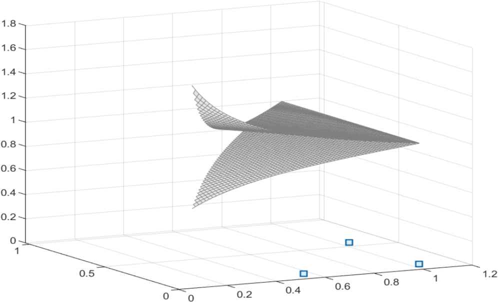
has always a zero and thus in the numerical examples we consider α < β. If we further consider β − α > 0.1 then η1η2<η2η1 and graphs of the functions (in α, β) are plotted in Fig. 1.
Fig. 1.
η1η2 the top and η2η1 the bottom functions as functions of α > β + 0.1
The deviation is bigger for smaller values of both parameters and approaches ∞ when α approaches β.
For the numerical estimates we pick values for β and α.
The case of chasing solitons: We pick α=π5 and β=π12 then
n2=−0.2588<m2=0.1045<m1=0.8090<n1=0.9659,
p1 = 0.3522 and p2 = 0.6124. The shifts are u = 0.1562, v = 0.2636, and k=0.0623ψ12+0.1882ψ22 while b=0.−568φ12+0.1718φ22+0.0002B2 and 0.9232⩽KB⩽1.0832.
The case of solitons traveling in opposite directions: We pick α=π24 and β=π6 then
m1=−0.6088<m2=0.3827<n2=0<n1=0.8660,
p1 = −0.1130 and p2 = 0.4330. The shifts are u = −0.1577, v = −0.5169, and k=0.0045ψ12+0.0655ψ22 while b=0.0167φ12+0.2456φ22+0.0110B2 and 0.7189⩽KB⩽1.0899.
The two examples illustrate that the interaction therm 1B2≈1K2 is the significant difference between 2-soliton solution for gB and KdV type potentials. The solitons corresponding to this term are virtual solitons in the context of [8]
. Visual inspection of 2-soliton solutions for the Euler’s equations, [16] confirmed that the presence of the interaction is relevant.
6. Discussion and Conclusions
In the previous sections we presented decomposition of the KdV type potentials, which include the 2-soliton solutions of KdV, as k=γ1(ψ1*)2+γ2(ψ2*)2 where, γi are constants depending only on p1, p2. The two functions ψi are eigenfunctions of ψxx = (λ2
− k*)ψ for eigenvalues p12, p22 and can be considered as two eigenstates, ψ1* excited and ψ2* steady state. In theorem 3.1, (3.4), we showed that b=h1Φ12+h2Φ22, where Φi are solutions of the transport-eigenvalue equations Φt + 2RΦx = Φxx + (−λ2
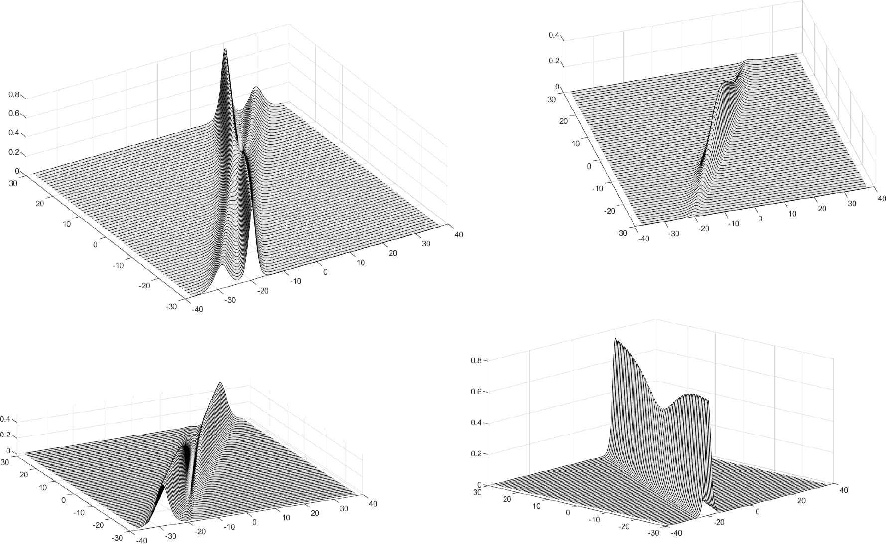
+ v)Φ and h1 and h2 are variable coefficients. In theorem 3.2 we established that b≈k*+1K2. A close examination of the formulas also shows that for the positive components ϕi ≈ ψi for i = 1, 2. The 2-soliton solution for gB can be considered as an energy transport process of two energy waves with influence on each other via the eigenfunctions ψi. For t → ±∞ the components Φi and ψi for i = 1, 2 correspondingly are bell-shaped and differ from the single soliton case primarily by a phase shift and the interaction terms tend to 0. From the signs of b1, b2 it also can be observed that during the interaction the two waves exchange energy, this might be concluded from the signs of the interaction terms and the fact that Φ1 has negative values. The dynamics is different for the solitons traveling in the same or opposite directions. In the case of chasing solitons, the two pairs of components are almost identical and the interaction results in loss of energy at the pick of ψ2* and energy gain away of it, as also can be seen from Fig. 2. In the case of opposite directions the interactions causes a temporarily appearance of a traveling wave along ψ1*, this agrees with the different signs of b1 and b2, as also can be seen from Fig. 3.
Fig. 2.
α=π5 and β=π12top left: superposition of k, lighter cooler, and b, black counter lines; top right: superposition of normalized interaction terms; bottom left: smaller component of v; bottom right: larger component of v.
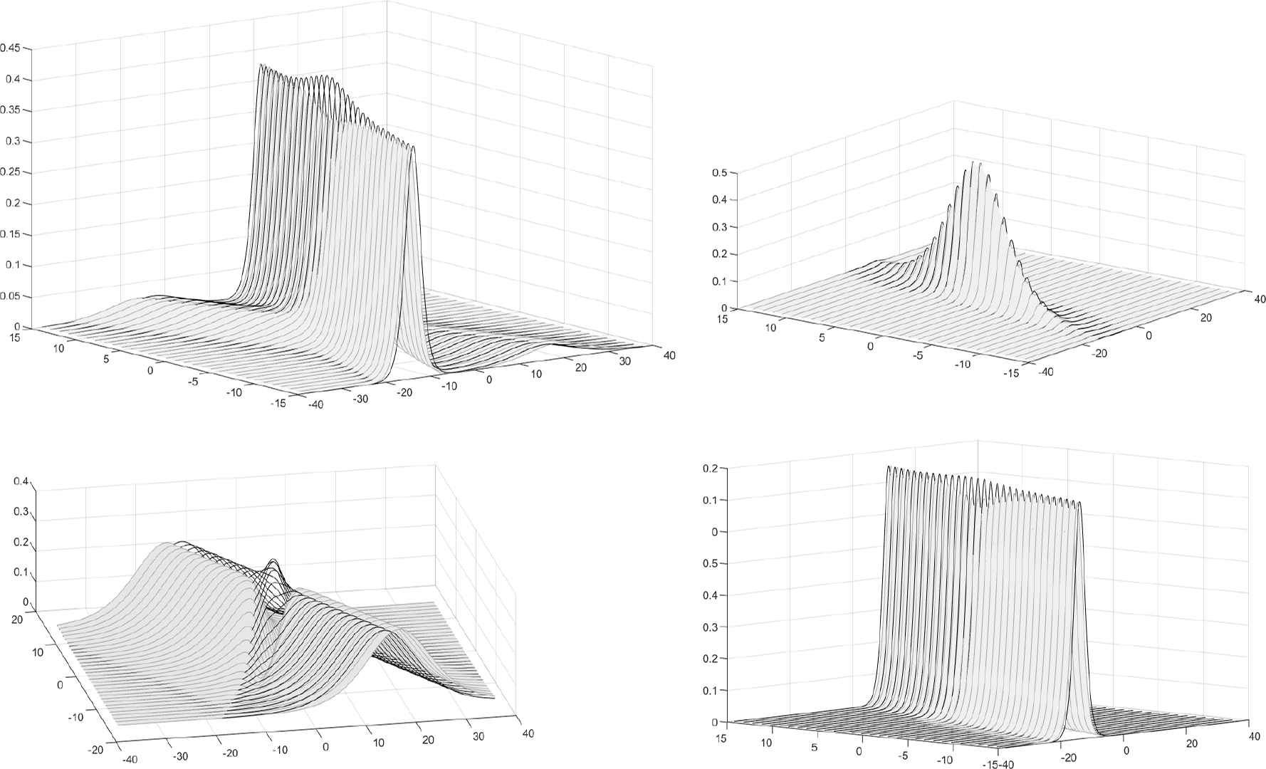
Fig. 3.
α=π24 and β=π6top left: superposition of k, lighter cooler, and b, black counter lines; top right: superposition of normalized interaction terms; bottom left: smaller component of v; bottom right: larger component of v.
Another observation that can be made is that ψ1 away from the interaction is up to a phase shift a single soliton while during the interaction it looks like transition from a steady state to excited state. This also might be in agreement with the fact that after interaction the smaller and slower soliton, ψ1, exhibits a time delay while the faster and taller, ψ2 exhibits positive time shift. The horizontal velocity of a particle is approximated by kdv and the slowing of the horizontal velocityof ψ1 can be explained by the more chaotic movement during the interaction while the acceleration in horizontal direction of ψ2 might be explained with the fact that the vertical displacement is lesser during interaction while the horizontal is about the same.
An interesting observation is that the results obtained in this work can be extended for gB type potentials b˜=2(lnV˜)xx. The Wronskian V˜=|f˜g˜f˜xg˜x| is generated by more general seed solutions
for arbitrary parameters (ai,j, bi,j), εj, i, j = 1, 2. Straight substitution and computations lead to similar decomposition as in theorem 3.1. The main difference is that the corresponding modes f˜V˜ and g˜V˜ are solutions to different type equations. This observation can be used to investigate 2-soliton solution for SWW equations with third order spatial eigenvalues, CH, DP, or N, equations for example.
Acknowledgement
An anonymous reviewer is thanked for critically reading the manuscript and suggesting important improvements.
[12]W.-X. Ma and Y. You, Solving the Korteweg-de Vries Equation by its Bilinear Form: Wronskian Solutions, Trans. of AMS, Vol. 357, No. 5, 2004, pp. 1753-1778.
[17]A.G. Rasin and J. Schiff, Unfamiliar Aspects of Backlund Transformations and an Associated Degasperis- Procesi Equation, Theor. Math. Phys, Vol. 196, 2018, pp. 1333-1346.
[23]B. Xia, R. Zhou, and Z. Qiao, Darboux transformation and multi-soliton solutions of the Camassa-Holm equation and modified Camassa-Holm equation, J. of Math. Phys, Vol. 57, 2016.
TY  - JOUR
AU  - Vesselin Vatchev
PY  - 2020
DA  - 2020/09/04
TI  - Decomposition of 2-Soliton Solutions for the Good Boussinesq Equations
JO  - Journal of Nonlinear Mathematical Physics
SP  - 647
EP  - 663
VL  - 27
IS  - 4
SN  - 1776-0852
UR  - https://doi.org/10.1080/14029251.2020.1819610
DO  - 10.1080/14029251.2020.1819610
ID  - Vatchev2020
ER  -