Journal of Nonlinear Mathematical Physics

Volume 27, Issue 4, September 2020, Pages 529 - 549

Minimal surfaces associated with orthogonal polynomials

Authors
Vincent Chalifour
Departement of mathematics and statistics, Université de Montréal, C. P. 6128, Succ. Centre-ville, Montréal, Québec, H3C 3J7, Canada,chalifour@dms.umontreal.ca
Alfred Michel Grundland*
1Centre de Recherches Mathématiques, Université de Montréal, C. P. 6128, Succ. Centre-ville, Montréal, Québec, H3C 3J7, Canada
2Departement of Mathematics and Computer Science, Université du Québec, CP500, Trois-Rivières, Québec, G9A 5H7, Canada,grundlan@crm.umontreal.ca
*Corresponding author.
Corresponding Author
Alfred Michel Grundland
Received 17 January 2019, Accepted 3 December 2019, Available Online 4 September 2020.
DOI
10.1080/14029251.2020.1819599How to use a DOI?
Keywords
Integrable system; soliton surface; minimal surface; orthogonal polynomial; Weierstrass immersion formula; Sym-Tafel immersion formula; CMC surface
Abstract

This paper is devoted to a study of the connection between the immersion functions of two-dimensional surfaces in Euclidean or hyperbolic spaces and classical orthogonal polynomials. After a brief description of the soliton surfaces approach defined by the Enneper-Weierstrass formula for immersion and the solutions of the Gauss-Weingarten equations for moving frames, we derive the three-dimensional numerical representation for these polynomials. We illustrate the theoretical results for several examples, including the Bessel, Legendre, Laguerre, Chebyshev and Jacobi functions. In each case, we generate a numerical representation of the surface using the Mathematica symbolic software.

Copyright
© 2020 The Authors. Published by Atlantis Press and Taylor & Francis
Open Access
This is an open access article distributed under the CC BY-NC 4.0 license (http://creativecommons.org/licenses/by-nc/4.0/).

1. Introduction

To describe the behavior of a continuous medium (fluid, gas or solid), theoretical physics uses various models, most of which lead to nonlinear partial differential equations (PDEs). The study of the general properties of these nonlinear equations and of the methods for solving them is a rapidly developing area of modern mathematics. Specifically, this is true in the study of integrable models in two independent variables, which have generated a great deal of interest and activity in several mathematical as well as physical fields of research. In particular, surfaces immersed in Lie groups, Lie algebras and homogeneous spaces which are associated with these models have been shown to play an essential role in several applications to nonlinear phenomena in diverse areas of physics, chemistry and biology (see e.g. [110] and references therein). An algebraic approach to the structural equations of these surfaces (i.e. the Gauss-Weingarten (GW) and Gauss-Codazzi (GC) equations) has often been very difficult to carry out. A geometrical approach to the derivation and classification of such systems, which we propose here for special functions, seems to be of importance for applications in several branches of science. The construction and investigation of two-dimensional (2D) surfaces obtained through the use of the soliton surface technique [11] allows the plotting of these functions, which constitutes the main objective of this work. We examine certain aspects of a visual image of surfaces reflecting the behavior of some special functions, focusing mainly on such functions as the Bessel, Legendre, Laguerre, Chebyshev and Jacobi functions and the associated series [1216], which can be of interest. This may provide some clues about the properties of these surfaces, which are otherwise hidden in some implicit mathematical expressions. This is, in short, the main topic of investigation.

The paper is organized as follows. Section 2 contains a brief summary of the results concerning the construction of minimal and constant mean curvature lambda (CMC-λ) surfaces (H = λ) immersed in the three-dimensional (3D) Euclidean and hyperbolic spaces, respectively. It is shown that the use of successive gauge transformations allows us to reduce the GW system of equations for the moving frame on these surfaces to a single linear second-order ordinary differential equation (ODE). The coefficients of this ODE are expressed in terms of two arbitrary holomorphic functions. Comparing them with the coefficients of the ODE associated with orthogonal polynomials allows us to construct their associated 2D-surfaces. It is shown that these surfaces are defined by the Weierstrass formula for immersion. The properties of surfaces associated with these polynomials are discussed in detail. In section 3, we illustrate the theoretical considerations for several classical orthogonal polynomials. We summarize the obtained results in tables 1 to 8. This analysis includes explicit solutions of the GW system, that is the wavefunctions and their potential matrices. For each orthogonal polynomial, a 3D numerical representation is constructed and investigated. The last section contains remarks and suggestions regarding possible further developements.

The Legendre equation: (1z2)d2ωdz22zdωdz+α(α+1)ω=0, α ∈ ℕ, z ≠ ±1.
η2=c121z2,χ=1λΔ1z+c2c12.
u11=u22=Δ1z+c21z2,u12=λc121z2,u21=1λ(Δ1z+c2)2c12(1z2).
Ψ1=k1Pα(z)+k2Qα(z),Ψ2=1λc12[k1(Pα(z)(Δ2z+c2)αPα1(z))+k2(Qα(z)(Δ2z+c2)αQα1(z))].
F1=14λ2e(1c14[Δ3(ϕ1ϕ2)+2Δ12z]ξ0ξ),F2=14λ2𝕀m(1c14[Δ3(ϕ1ϕ2)2Δ12z]ξ0ξ),F31=12λe([(Δ1c2)ϕ2+(Δ1+c2)ϕ1]ξ0ξ).
F˜11=F˜22=i4λ([(Δ1c2)ϕ2+(Δ1+c2)ϕ1]ξ0ξ([(Δ1c2)ϕ2+(Δ1+c2)ϕ1]ξ0ξ)*)F˜12=i4(c12[ϕ1ϕ2]ξ0ξ1λ2(1c14[(Δ1+c2)2ϕ1(Δ1c2)2ϕ22Δ12z]ξ0ξ)*)F˜21=i4(1λ2c14[(Δ1+c2)2ϕ1(Δ1c)2ϕ22Δ12z]ξ0ξ(c12[ϕ1ϕ2]ξ0ξ)*).

Note: Pα, Qα : αth-order Legendre polynomials, 1st and 2nd kind.

Δ1 = α(α + 1), Δ2 = α(α + 2), Δ3=λ2c14(α(α+1)+c2)2, ϕ1 = log(1 + z), ϕ2 = log(1 − z).

Table 1:

Summary. The Legendre equation

The Legendre associated equation: (1z2)d2ωdz22zdωdz+(α(α+1)m21z2) ω = 0, α, m ∈ ℕ, m ≠ 0, z ≠ ±1.
η2=c121z2,χ=1λm22(ϕ1ϕ2)Δz+c2c12.
u11=u22=Δ1z+c21z2,u12=λc121z2,u21=1λ(Δ1z+c2)2c12(1z2).
Ψ1=k1Pαm(z)+k2Qαm(z),Ψ2=1λc12[(m22(ϕ1ϕ2)Δz+c2)[k1Pαm(z)+k2Qαm(z)]+k1(z21)m/22αα!(mzdm+αdzm+α(z21)α+(z21)dm+α+1dzm+α+1(z21)α+k2(z21)m/2(mzdmdzmQα(z)+(z21)dm+1dzm+1Qα(z)))].
F1=12Re([c122(ϕ1ϕ2)124λ2c12(24(α2+2α3+α4)z+12(c22+2c2α+α2+2c2α2+2α3+α4)ϕ1+6m2(c2+Δ)ϕ12+m4ϕ13+3m2ϕ22(2c22Δ+m2ϕ1)m4ϕ23ϕ2(12c2224c2Δ+Δ(12Δ7,225m2)+12m2(c2+Δ)ϕ1+3m4ϕ12)24m2ΔLi2((1z)/2))]ξ0ξ),F2=12Im([c122(ϕ1ϕ2)+124λ2c12(24(α2+2α3+α4)z+12(c22+2c2α+α2+2c2α2+2α3+α4)ϕ1+6m2(c2+Δ)ϕ12+m4ϕ13+3m2ϕ22(2c22Δ+m2ϕ1)m4ϕ23ϕ2(12c2224c2Δ+Δ(12Δ7,225m2)+12m2(c2+Δ)ϕ1+3m4ϕ12)24m2ΔLi2((1z)/2))]ξ0ξ),F3=18λRe([m2ϕ22+ϕ1(4(Δc2)2m2ϕ1)+ϕ1(4(Δ+c2)+m2ϕ1)]ξ0ξ).
F˜11=F˜22=i16λ([m2ϕ22+ϕ2(4(Δc2)2m2ϕ1)+ϕ1(4(Δ+c2)+m2ϕ1)]ξ0ξ+([m2ϕ22+ϕ2(4(Δc2)2m2ϕ1)+ϕ1(4(Δ+c2)+m2ϕ1)]ξ0ξ)*),F˜12=i4([c12(ϕ1ϕ2)]ξ0ξ112λ2(1c12[(24(α2+2α3+α4)z+12(c22+2c2α+(2c2+1)α2+2α3+α4)ϕ1+6m2(c2+Δ)ϕ12+m4ϕ13+3m2ϕ22(2c22Δ+m2ϕ1)m4ϕ23ϕ2(12c22+Δ(12Δ7,225m224c2)+12m2(c2+Δ)ϕ1+3m4ϕ12)24m2ΔLi2((1z)/2))]ξ0ξ)*),F˜21=i4(112λ2c12[24(α2+2α3+α4)z+12(c22+2c2α+(2c2+1)α2+2α3+α4)ϕ1+6m2(c2+Δ)ϕ12+m4ϕ13+3m2ϕ22(2c22Δ+m2ϕ1)m4ϕ23ϕ2(12c22+Δ(12Δ,7,255m224c2)+12m2(c2+Δ)ϕ1+3m4ϕ12)24m2ΔLi2((1z/2)]ξ0ξ+([c12(ϕ1ϕ2)]ξ0ξ)*).

Note: Pαm, Qαm: αth-order Associated Legendre functions of degree m, 1st and 2nd kind, Li2: Polylogarithm function.

Δ = α(α + 1), ϕ1 = log(1 + z), ϕ2 = log(1 − z).

Table 2:

Summary. The Legendre associated equation

The Bessel equation: z2d2ωdz2+zdωdz+(z2p2)ω=0, p ∈ ℂ.
η2=c1z1,χ=1λc1(p2log(z)z22+c2).
u11=u22=1z(p2log(z)z22+c2),u12=λc1z,u21=1λc11z(p2log(z)z22+c2)2.
Ψ1=k1𝒥p(z)+k2𝒴p(z),Ψ2=1λc1[k1(z2𝒥p1(z)+(p2log(z)z22+c2)𝒥p(z)+z2𝒥p+1(z))+k2(𝒴p1(z)+(p2log(z)z22+c2)𝒴p(z)𝒴p+1(z))].
F1=12λ2Re(1c1[(λ2c12c22+p2z22)log(z)c2p2log2(z)p43log3(z)(4p28c2+z2)z216]ξ0ξ),F2=12λ2Im(1c1[(λ2c12c22p2z22)log(z)+c2p2log2(z)+p43log3(z)+(4p28c2+z2)z216]ξ0ξ),F3=1λRe([c2log(z)+p22log2(z)z24]ξ0ξ).
F˜11=F˜22=i2λ(ϕ+ϕ*),F˜12=i2(c1log(z)|ξ0ξ1λ2(1c1[log(z)(c22p2z22)+z216(8c2+4p2+z2)+c2p2log2(z)+p43log3(z)]ξ0ξ)*)F˜21=i2(1λ2c1[(log(z)(c22p2z22)+z216(8c2+4p2+z2)+c2p2log2(z)+p43log3(z))]ξ0ξ(c1log(z)|ξ0ξ)*).

Note: 𝒥p, 𝒴p: p th-order Bessel functions, 1st and 2nd kind. ϕ=[p22log2(z)z24+c2log(z)]ξ0ξ.

Table 3:

Summary. The Bessel equation

The Chebyshev equation of the 1st kinda: (1z2)d2ωdz2zdωdz+n2ω=0, n ∈ ℕ, z ≠ ±1.
η2=c11z2,χ=1λn2ϕ+c2c1.
u11=u22=n2ϕ+c21z2,u12=λc11z2,u21=1λ(n2ϕ+c2)2c1(1z2).
Ψ1=k1Tn(z)+k21z2T2,n1(z),Ψ2=1λc(k1(n2arcsin(z)+c1)Tn(z)+k1(n+1)1z2Tn2(z)+(k2(n2arcsin(z)+c1)1z2+k1n2k2z1z2)T2,n1).
F1=12Re(1λ2c1[(λ2c12c22)ϕ+n2c2ϕ2n43ϕ3]ξ0ξ),F2=12Im(1λ2c1[(λ2c12+c22)ϕn2c2ϕ2+n43ϕ3]ξ0ξ),F3=1λRe([c2ϕ+n22ϕ2]ξ0ξ).
F˜11=F˜22=i2λ([c2ϕ+n22ϕ2]ξ0ξ+([c2ϕ+n22ϕ2]ξ0ξ)*),F˜12=c1i2ϕ|ξ0ξ+i2λ2(1c1[c22ϕn2c2ϕ2+n43ϕ3]ξ0ξ)*,F˜21=i2λ2c1[c22ϕn2c2ϕ2+n43ϕ3]ξ0ξi2(c1ϕ|ξ0ξ)*.

Note: Tn, T2,n: Chebyshev polynomials, 1st and 2nd kind. ϕ = arcsin(z).

a

To obtain the results for the Chebyshev equation of the 2nd kind, we perform the transformation nnn+2.

Table 4:

Summary. The Chebyshev equations

The Laguerre associated equation: zd2ωdz2+(α+1z)dωdz+nω=0, α, n ∈ ℕ, z ≠0.
η2=ezc1zα+1,χ=1λ(nc1ϕ1+c2).
u11=u22=nc1ϕ1+c2c1zα+1ez,u12=λezc1zα+1,u21=1λ(nc1ϕ1+c2)2c1zα+1ez.
Ψ1=k1Lnα(z)+k2U(n,α+1,z),Ψ2=1λ[k1(((nc1ϕ1+c2)nc1zαez)Lnα(z)+(n+α)c1zα+1ezLn1α(z))+k2((nc1ϕ1+c2)U(n,α+1,z)nc1zα+1ezU(n+1,α+2,z))].
F1=12Re(1λ2[n2c1(α!)2p=0αq=0αΓ(p+qα,z)p!q!+1c1(c22λ2)zαEα+1(z)2nc2ϕ2]ξ0ξ),F2=12Im(1λ2[n2c1(α!)2p=0αq=0αΓ(p+qα,z)p!q!1c1(λ2+c22)zαEα+1(z)+2nc2ϕ2]ξ0ξ),F3=1λRe([nϕ2c2c1zαEα+1(z)]ξ0ξ).
F˜11=F˜22=i2λ([nϕ2c2c1zαEα+1(z)]ξ0ξ+([nϕ2c2c1zαEα+1(z)]ξ0ξ)*),F˜12=i2(1c1zαEα+1(z)|ξ0ξ+1λ2([n2c1(α!)2p=0αq=0αΓ(p+qα,z)p!q!c22c1zαEα+1(z)+2nc2ϕ2]ξ0ξ)*),F˜21=i2(1λ2[n2c1(α!)2p=0αq=0αΓ(p+qα,z)p!q!c22c1zαEα+1(z)+2nc2ϕ2]ξ0ξ+(1c1zαEα+1(z)|ξ0ξ)*).

Note: Γ(ν, z): Incomplete gamma function, Lnα: Associated Laguerre polynomial, U(ν1, ν2, z): Hypergeometric function, 2nd kind, Em: Exponential integral m-function. ϕ1 = Γ(α + 1, z), ϕ2=α!r=0α1zrαr!(rα)+log(z).

Table 5:

Summary. The Laguerre associated equation

The Hermite equation: d2ωdz22zdωdz2nω=0, n ∈ 𝕑.
η2=c12ez2,χ=2nλc12z0zes2ds.
u11=u22=2nez2z0zes2ds,u12=λc12ez2,u21=4n2λc12ez2(z0zes2ds)2.
Ψ1=k1Hn(z)+k2F11(n2,12,z2),Ψ2=2nλc1(k1(ez2c1Hn1(z)Hn(z))k2(F11(n2+1,32,z2)+F11(n2,12,z2)z0zes2ds)).
F1=12Re(c12ξ0ξ(1(2nλc12z0zes2ds)2)ez2dz),F2=12Im(c12ξ0ξ(1+(2nλc12z0zes2ds)2)ez2dz),F3=2nλRe(ξ0ξz0zes2dsez2dz).
F˜11=F˜22=niλ(ξ0ξz0zes2dsez2dz+(ξ0ξz0zes2dsez2dz*)),F˜12=i2(c12ξ0ξez2dz4n2λ2(1c12ξ0ξ(z0zes2ds)2ez2dz)*),F˜21=i2(4n2λ2c12ξ0ξ(z0zes2ds)2ez2dz(c12ξ0ξez2dz)*).

Note: Hn: nth-order Hermite polynomial, pFq: Hypergeometric function.

Table 6:

Summary. The Hermite equation

The Gegenbauer equation: (1z2)d2ωdz2(2α+1)dωdz+n(n+2α)ω=0, n ∈ ℕ, α ∈ ℂ, z ≠ ±1.
η2=c1(1+z1z)α+1/2,χ=1λΔ2(1z)α+1/2(1+z)α1/2+c2c1Δ3.
u11=u22=Δ2+c2(1+z1z)α+1/2Δ3,u12=λc1(1+z1z)α+1/2,u21=1λΔ22(1z1+z)α+1/2+2c2Δ2+c22(1+z1z)α+1/2c1Δ32.
Ψ1=k1ϕ1+k22α1/2(z1)α+1/2ϕ2,Ψ2=1λc1[k1(Δ2(1z1+z)α+1/2+c2Δ3ϕ1+14(Δ1+1)(Δ11)α+1/2(1z1+z)Δ3/4ϕ3)+k22α1/2(z1)1/2α((Δ2(1z1+z)α+1/2+c2Δ3+(1/2α)(z1)1)ϕ212Δ1(α+1/4Δ1)3/2αϕ4)].
F1=12Re([c121/2α2α+3ϕ51λ2c1Δ32(Δ222α+3/212α(1+z)1/2αϕ6+c2221/2α2α+3ϕ5+2c2Δ2z)]ξ0ξ),F1=12Im([c121/2α2α+3ϕ5+1λ2c1Δ32(Δ222α+3/212α(1+z)1/2αϕ6+c2221/2α2α+3ϕ5+2c2Δ2z)]ξ0ξ),F3=1λRe(1Δ3[Δ2z+c221/2α2α+3ϕ5]ξ0ξ).
F˜11=F˜22=i2λ(1Δ3[Δ2z+c221/2α2α+3ϕ5]ξ0ξ+(1Δ3[Δ2z+c221/2α2α+3ϕ5]ξ0ξ)*),F˜12=i2([c121/2α2α+3ϕ5]ξ0ξ1Δ3(1c1Δ32[Δ222α+3/212α(1+z)1/2αϕ6+c2221/2α2α+3ϕ5+2c2Δ2z]ξ0ξ)*).F˜21=i2(1λ2c1Δ32[Δ222α+3/212α(1+z)1/2αϕ6+c2221/2α2α+3ϕ5+2c2Δ2z]ξ0ξ([c121/2α2α+3ϕ5]ξ0ξ)*).

Note: pFq: Hypergeometric function. Δ1=4n2+8αn+1, Δ2 = n(n + 2α), Δ3 = 2α + 1.

ϕ1=F21(1/2(Δ1+1),1/2(Δ11);α+1/2;1z2), ϕ2=F21(α1/2Δ1,1/2Δ1;3/2α;1z2), ϕ3=F21(11/2(Δ1+1),1+1/2(Δ11);α+3/2;1z2), ϕ4=F21(1α1/2Δ1,1+1/2Δ1;5/2α;1z2), ϕ5=(1+z)α+3/2F21(α+1/2,α+3/2;α+5/2;1+z2), ϕ6=F21(α1/2,1/2α;3/2α;1+z2).

Table 7:

Summary. The Gegenbauer equation

The Jacobi eq.: (1z2)d2ωdz2+(βα(α+β+2)z)dωdz+n(n+α+β+1)ω=0 n ∈ ℕ, α, β ∈ ℂ, z ≠ ±1.
η2=c1(1+z)(β+1)(1z)(α+1),χ=1λΔ(z+1)β+1ϕ3+c2c1(β+1).
u11=u22=Δ(z+1)β+1ϕ3+c2(β+1)(1+z)β+1(1z)α+1,u12=λc1(1+z)β+1(1z)α+1,u21=1λ(Δ(z+1)β+1ϕ3+c2)2c1(β+1)2(1+z)β+1(1z)α+1.
Ψ1=k1ϕ1+2αk2(z1)αϕ2,Ψ2=1λc1[k1Δ2α(2α(z+1)β+1ϕ3+c2β+1ϕ1+12(α+1)(1+z)β+1(1z)α+1ϕ4)+k2(2αΔ2α(z+1)β+1ϕ3+c2β+1(z1)αϕ2+2α(1)α(α(1+z)β+1ϕ2+(α+n)(β+n+1)2(α1)(1+z)β+1(1z)ϕ5))].
F1=12Re(c12α+2(1+z)β(1+z1zϕ62βϕ7)1λ2c1[Δ22α(β+1)]2ϕ10c222α+2(z+1)β(z+1β1ϕ6+2βϕ7)2c2Δ(β+1)ϕ8),F2=12Im(c12α+2(1+z)β(1+z1zϕ62βϕ7)+1λ2c1[Δ22α(β+1)2ϕ10c222α+2(z+1)β(z+1β1ϕ6+2βϕ7)2c2Δ(β+1)ϕ8]),F3=1λRe(1(β+1)[Δ2α(β+1)ϕ9c22α+2(z+1)β(z+1β1ϕ6+2βϕ7)]).
F˜11=F˜22=i2λ(1(β+1)[Δ2α(β+1)ϕ9c22α+2(z+1)β(z+1β1ϕ6+2βϕ7)]ξ0ξ+(1(β+1)[Δ2α(β+1)ϕ9c22α+2(z+1)β(z+1β1ϕ62βϕ7)]ξ0ξ)*),F˜12=i2(c12α+2[(1+z)β(1+z1zϕ6+2βϕ7)]ξ0ξ+1λ2(1c1[Δ22α(β+1)2ϕ10c222α+2(z+1)β(z+1β1ϕ6+2βϕ7)2c2Δ(β+1)ϕ8]ξ0ξ)*),F˜21=i2(1λ2c1[Δ22α(β+1)2ϕ10c222α+2(z+1)β(z+1β1ϕ6+2βϕ7)2c2Δ(β+1)ϕ8]ξ0ξ+(c12α+2[(1+z)β(1+z1zϕ6+2βϕ7)]ξ0ξ)*).

Note: pFq: Hypergeometric function. DomainJacobi = {ξ ∈ ℂ | |ξ| < 1 and |ξ + 1| < 2|α|}.

Δ = 2α n(n + α + β + 1), ϕ1=F21(n,α+β+n+1;α+1;1z2), ϕ2=F21(αn,β+n+1;1α;1z2), ϕ3=F21(α,β+1;β+2;1z2), ϕ4=F21(1n,α+β+n+2;α+2;1z2), ϕ5=F21(αn+1,β+n+2;2α;1z2), ϕ6=F21(1β,α+1;2β;1+z2), ϕ7=F21(β,α;1β;1+z2), ϕ8=s=0((α)s(z+1)s+1(β+s+1)(s+1)s!2s+2α+1F21(s+1,α+1;s+2;1+z2)), ϕ9=s=0((α)s(z+1)s+1(β+s+1)(s+1)s!2s+1F21(s+1,α+1;s+2;1+z2)), ϕ10=s=0k=0((α)s(α)k(z+1)s+k+β+1(β+s+1)(β+k+1)(β+s+k+1)s!k!2s+k(F21(s+k+β+1,α+1;s+k+β+2;1+z2)F21(s+k+β+1,α;s+k+β+2;1+z2)))..

Table 8:

Summary. The Jacobi equation

2. Linear problem and immersion formulas

In this section, according to [17] , we recall the main concepts required to study the linear problem (LP) related to the GW equations for frames on 2D-surfaces, which are the Enneper-Weierstrass and Sym-Tafel formulas for immersion, both in Euclidean and hyperbolic spaces. We make use of the gauge transformations in order to reduce the LP to a single linear second-order ODE and to investigate its links with orthogonal polynomials.

2.1. The linear problem for minimal surfaces

To make the paper self-contained, we summarize the basic facts on the immerson of minimal surfaces in the Euclidean space 𝔼3 given in [11,18], together with the quaternionic description of these surfaces in the 𝔰𝔲(2) algebra. Let F be a smooth orientable and simply-connected surface in 𝔼3 given by a vector-valued function

F=(F1,F2,F3)T:𝔼3(2.1)
where is a Riemann surface. A conformally parametrized surface involving complex coordinates z and z¯ requires that the tangent vectors ∂F, ¯F and the unit normal N satisfy the following normalization
(F|F)=0,(¯F|¯F)=0,(F|¯F)=12eu,(2.2)
(F|N)=0,(¯F|N)=0,(N|N)=1,(2.3)
where u is a real-valued function u : → ℝ. The brackets (· | ·) denote the scalar product in 𝔼3
(a|b)=i=13aibi.(2.4)

We have used the notation for the holomorphic and antiholomorphic derivatives

=12(xiy),¯=12(x+iy),z=x+iy.(2.5)

The Hopf differential Qdz on and the mean curvature on F are defined by

Q=(2F|N),H=2eu(¯F|N),(2.6)
respectively. For a minimal surface (H = 0), the GW equations for a moving frame σ = (∂F, ¯F, N)T take the form
σ=𝒰σ,¯σ=𝒱σ,(2.7)
where
𝒰=(u0Q00002eu0),𝒱=(0000¯uQ¯2euQ¯00).(2.8)

The compatibility conditions of the GW equations (2.7), often called the Zero-Curvature Condition (ZCC)

¯𝒰𝒱+[𝒰,𝒱]=0,(2.9)
are reduced to the GC equations
¯u2|Q|2eu=0,¯Q=0,(2.10)
where Q is a holomorphic function of z. It is convenient to use the Lie algebra isomorphism 𝔰𝔬(3) ≃ 𝔰𝔲(2) and to write the GW equations in terms of 2 × 2 matrices
Φ=𝒰Φ,¯Φ=𝒱Φ,(2.11)
where
𝒰=(14uQeu2014u),𝒱=(14¯u0Q¯eu214¯u)𝔰𝔩(2,).(2.12)

Here 𝒱 = −𝒰 is an anti-Hermitian matrix.

The Enneper-Weierstrass immersion formula for minimal surfaces is defined by the contour integral [19, 20]

F=(12ez0z(1χ2)η2dξ,12𝕀mz0z(1+χ2)η2dξ,ez0zχη2dξ)T𝔼3,(2.13)
in terms of two holomorphic functions η and χ, i.e. ¯η=¯χ=0. Equations (2.11) can be reduced to two equations expressed in terms of these two holomorphic functions. We apply the gauge transformation M to the wavefunction Φ in equations (2.11) as proposed in [17] , i.e.
Ψ=MΦ,whereM=(|η|(1+χχ¯)1/2ηχ0|η|η(1+χχ¯)1/2ηχ|η|(1+χχ¯)1/2)SL(2,).(2.14)

We obtain

Ψ=λη2(χ1χ2χ)Ψ,¯Ψ=0,(2.15)
where
𝒰(λ;z)=λη2(χ1χ2χ)𝔰𝔲(2).(2.16)

Note that Ψ is a holomorphic function and 𝒰 is parametrized by λ ∈ ℂ\{0}. The wavefunction Φ in (2.11) can also be expressed in terms of the holomorphic functions η and χ

Φ=1(1+χχ¯)1/2(χeiθeiθeiθχ¯eiθ)SU(2),(2.17)
where η = re, r ∈ ℝ+, θ ∈ [0, 2π[ and λ=η/η¯=e2iθ is the spectral parameter. The Sym-Tafel type formula FST for the immersion of a 2D-surface in 𝔰𝔲(2) ≃ 𝔼3 is given by [21, 22]
FST=Φ1λΦ=i1+χχ¯(1χχ¯2χ¯2χ1+χχ¯),¯χ=0.(2.18)

Let F˜ be the quaternionic description of the Enneper-Weierstrass formula (2.13). In view of the isomorphism 𝔰𝔬(3) ≃ 𝔰𝔲(2), the Enneper-Weierstrass formula (2.13) for the immersion of minimal surfaces takes the form

F˜=i2(z0zχη2dξ+(z0zχη2dξ)*z0zη2dξ(z0zχ2η2dξ)*z0zχ2η2dξ+(z0zη2dξ)*z0zχη2dξ(z0zχη2dξ)*)𝔰𝔲(2),(2.19)
where * denotes the complex conjugate of the considered expression.

2.2. Immersion in the hyperbolic space H3(((λ))) of curvature λ

In this section, we use results from the soliton approach [11,22,23] for the study of CMC surfaces in the hyperbolic space H3(λ). Consider the conformal immersion of surfaces in the hyperbolic space

Fσ:H3(λ)3,1,(2.20)
where ℝ3,1 is the Lorentz space with standard bilinear form
(X|Y)=X1Y1+X2Y2+X3Y3X0Y0(2.21)
and the hyperboloid H3 is given by the scalar product
(X|X)=λ2.(2.22)

The conformality conditions are given by

(Fσ|Fσ)=0,(¯Fσ|¯Fσ)=0.(2.23)

The vectors Fσ, ∂Fσ, ¯Fσ and N form a moving frame σ = (Fσ, ∂Fσ, ¯Fσ, N)T on a surface which satisfies the following normalization relations

(Fσ|N)=0,(Fσ|N)=0,(¯Fσ|N)=0,(N|N)=1.(2.24)

We define the functions u, H and Q as in (2.6). The GW equations for the moving frame are given by

2Fσ=uFσ+QN,¯Fσ=λ22euFσ+12HeuN,N=HFσ2Qeu¯Fσ,(2.25)
and the GC equations take the form
¯u+12(H2λ2)eu2|Q|2eu=0,¯Q=12Heu,Q¯=12¯Heu.(2.26)

In the case of CMC-λ surfaces (H = λ), the reduced GC equations take the form [17]

¯u2|Q|2eu=0,¯Q=0,(2.27)
where Q is a holomorphic function. We note that equation (2.27), which is a Liouville type equation, coincides with the reduced form of the GC equations (2.10) obtained in the case of minimal surfaces (H = 0) immersed in the Euclidean space 𝔼3, with general solution
eu/2=ηη¯(1+χχ¯),Q=η2χ.(2.28)

The reduced linear problem associated with equations (2.26) takes the form

Φ=(14uQeu2λeu214u)Φ,¯Φ=(14¯u0Q¯eu214¯u)Φ.(2.29)

Let us identify the vector X ∈ ℝ3,1 with 2 × 2 Hermitian matrices using the Pauli matrices {σα}α=13 and the identity σ0 := 𝟙2 [24]

X=(X0,X1,X2,X3)Xσ=α=03Xασα=(X0+X3X1iX2X1+iX2X0X3).(2.30)

The scalar product is then given by

(X|Y)=12Tr(Xσiσ2(Yσ)Tiσ2),(2.31)
where (X | X) = −det(Xσ). We use the homomorphism
ρ:SL(2,)SO(3,1),(ρ(A)X)σ=AXσA.(2.32)

Consider Φ ∈ SL(2, ℂ) which transforms the orthonormal basis B = {𝟙2, σ1, σ2, σ3} into the orthonormal basis (the frame) B′ = {Fσ, ∂xFσ, ∂yFσ, N} by the relation

(λFσ,eu2xFσ,eu2yFσ,Nσ)=Φ(𝟙2,σ1,σ2,σ3)Φ.(2.33)

To study the LP, we define the potential matrices 𝒰, 𝒱 in the 𝔰𝔩(2, ℂ) algebra by

Φ=𝒰Φ,¯Φ=𝒱Φ.(2.34)

Therefore these matrices take the following explicit form [11]

𝒰=(14uQeu212eu2(λ+H)14u),𝒱=(14uQeu212eu2(λH)14u)𝔰𝔩(2,).(2.35)

Note that with the same gauge M (2.14), the gauge transformation process leads to the same structure, either with the transformation of the LP (2.11) associated with minimal surfaces immersed in the Euclidean space 𝔼3, or with the transformation of the LP (2.29) associated with CMC-λ surfaces immersed in the hyperbolic space H3(λ). Therefore, the linear system (2.15) can equivalently be expressed by the system

2Ψ12ηηΨ1λη2χΨ1=0,(2.36)
Ψ2=χΨ1Ψ1λη2,(2.37)
where Ψ = (Ψ1, Ψ2)T. The coefficients of the linear second-order ODE (2.36) possess a degree of freedom involving two arbitrary locally holomorphic functions η and χ. The complex-valued functions of one variable η(z) and χ(z) correspond to the arbitrary functions from the Enneper-Weierstrass representation (2.13) describing minimal surfaces in 𝔼3, which is equivalent to the Sym-Tafel formula (2.18) [25] .

From a solution Φ of the linear system (2.34), the formula

Fσ=1λΦΦH3(λ)(2.38)
represents a conformal immersion in H3(λ). In the limit λ → 0, we have H3(λ) → 𝔼3, but the denominator in (2.38) goes to infinity. To solve this problem, before taking the limit, we perform a translation by shifting the origin from the center of the hyperboloid to one of the points on the hyperboloid, applying a limiting procedure used in [17] , similar to the one proposed in [26]
F˜σ=limλ01λ(ϕϕ𝟙2).(2.39)

3. Special functions and associated soliton surfaces

In this section, we examine the ODE (2.36) in the case where it coincides with ODEs describing orthogonal polynomials. We present an example in which we solve the LP associated with the Laguerre polynomial. We discuss the explicit form of the Enneper-Weierstrass representation of 2D-surfaces immersed in 𝔼3 associated with this polynomial. Next, a summary of the results is presented for several classical orthogonal polynomials, under the form of tables, together with 3D images of selected surfaces.

3.1. The Laguerre equation: a complete example

The Laguerre equation for the unknown function ω takes the form

d2ωdz2+1zzdωdz+αzω=0,z0,α.(3.1)

Comparing the coefficients of (3.1) with those of (2.36), we obtain the explicit form of the meromorphic functions η and χ. In general, for an ODE of the form

p(ν;z)d2ρdz2+q(ν;z)dρdz+r(ν;z)ρ=0,p0,(3.2)
we obtain the relations
q(ν;z)p(ν;z)=2ηη,r(ν;z)q(ν;z)=λη2χ,(3.3)
where we abbreviate the notation for the dependence of a function f on the parameters of the ODE (3.2) by writing f (ν; z), ν:= (ν1, ν2,...,νn). For any second-order linear homogeneous ODE of the form (3.2), the meromorphic functions η and χ take the form
η(ν;z)=k1Exp{120zq(ν;ξ)p(ν;ξ)dξ},(3.4)
χ(ν;λ;z)=k2λExp{0zq(ν;ξ)p(ν;ξ)dξ}r(ν;z)p(ν;z)dz,(3.5)
where k1, k2 ∈ ℂ are arbitrary integration constants and λ ≠ 0 is the parameter of the LP (2.15). Making use of (3.3) for the Laguerre equation, we find
η2(z)=ezc1z,χ(α;λ;z)=1λ(αc1ez+c2),(3.6)
where c1 ∈ ℂ \ {0}, c2 ∈ ℂ are arbitrary integration constants and the functions η and χ are holomorphic, i.e. ¯η=¯χ=0. In view of (2.16), the potential matrix becomes
𝒰(α;λ;z)=(α+c2c1ezzλezc1z1λ(αc1ez+c2)2ezc1zα+c2c1ezz)𝔰𝔩(2,).(3.7)

Making use of (3.6), we eliminate η et χ from equation (2.36) and obtain the Laguerre equation with dependent variable Ψ1

zd2Ψ1dz2+(1z)dΨ1dz+αΨ1=0,z0,α.(3.8)

To determine the wavefunction Ψ which satisfies the LP (2.15), we solve (3.8) for its first component Ψ1

Ψ1=k1Lα(z)+k2U(α,1,z),k1,k2,(3.9)
where Lα(z) et U(−α,1, z) are, respectively, the αth-order Laguerre polynomial and the hypergeometric function of the second kind [15]. The general solution of the Laguerre equation (3.9) allows us to calculate the second component of the wavefunction Ψ2 from relation (2.37)
Ψ2=χΨ1Ψ1λη2=1λ[k1(c2Lα(z)+c1αezLα1(z))+k2((c1αez+c2)U(α,1,z)c1αzezU(1α,2,z))],(3.10)
where we use the well known recurrence formulas [15]
zddzLm(z)=mLm(z)mLm1(z),(3.11)
ddzU(ν1,ν2,z)=ν1U(ν1+1,ν2+1,z).(3.12)

The wavefunction Ψ associated with the LP (2.15) takes the form

Ψ(α;λ;z)=(k1Lα(z)+k2U(α,1,z)1λ[k1(c2Lα(z)+c1αezLα1(z))+k2((c1αez+c2)U(α,1,z)c1αzezU(1α,2,z))]),(3.13)
where z ≠ 0. We make use of (2.13) to calculate the Enneper-Weierstrass representation of the surface F ∈ 𝔼3. We find
F1(α;λ;ξ,ξ¯)=12Re(1λ2[1c1(λ2c22)Ei(z)α2c1Ei(z)2αc2log(z)]ξ0ξ),F2(α;λ;ξ,ξ¯)=12Im(1λ2[1c1(λ2+c22)Ei(z)+α2c1Ei(z)+2αc2log(z)]ξ0ξ),F3(α;λ;ξ,ξ¯)=Re(1λ[(αlog(z)+c2c1Ei(z))]ξ0ξ), (3.14)
where the notation |ξ0ξ means that the previous expression is evaluated from a constant ξ0 to an arbitrary complex number ξ. The function Ei(z) corresponds to the complex exponential integral as defined in [27]
Ei(z)=k=1zkkk!+12(log(z)log(1z))+γ,(3.15)
where γ is the Euler-Mascheroni constant. In view of (2.19), the components of the quaternionic representation F˜=(F˜ij) of the surface immersed in the 𝔰𝔲(2) algebra take the form
F1(α;λ;ξ,ξ¯)=12Re(1λ2[1c1(λ2c22)Ei(z)α2c1Ei(z)2αc2log(z)]ξ0ξ),F2(α;λ;ξ,ξ¯)=12Im(1λ2[1c1(λ2+c22)Ei(z)+α2c1Ei(z)+2αc2log(z)]ξ0ξ),F3(α;λ;ξ,ξ¯)=Re(1λ[(αlog(z)+c2c1Ei(z))]ξ0ξ), (3.16)

We simplify the problem to illustrate a particular case of the Laguerre equation and to show a numerical display of the surface in 𝔼3. Let α = 1. The Laguerre equation (3.1) becomes

zd2ωdz2+(1z)dωdz+ω=0(3.17)
and by comparing the coefficients of (3.17) with those of (2.36), we find the holomorphic functions as in (3.6). Considering fixed arbitrary integration constants and the parameter λ, let c1 = 1, c2 = 0, k1 = 1, k2 = 1 and λ = 1. From (3.3), the holomorphic functions η and χ become
η2(1;1;z)=ezz,χ(1;1;z)=ez,(3.18)
where ¯η=¯χ=0. The potential matrix (2.16) takes the form
𝒰(1;1;z)=1z(1ezez1)𝔰𝔩(2,)(3.19)
and the wavefunction takes the form
Ψ(1;1;z)=(Ψ1Ψ2)=((z1)(Ei(z)+1)ezez(Ei(z)+1)),(3.20)
where we use the relations (2.36) and (2.37). The second component Ψ2 was obtained using the differentiation formula [15]
ddzEi(z)=ezz.(3.21)

We verify that 𝒰 and Ψ are solutions of the LP (2.15) using the notation 𝒰Ψ := (Λ1, Λ2)T and verifying that ∂Ψ1 = Λ1, ∂Ψ2 = Λ2.

𝒰(λ,z)Ψ=(Λ1Λ2)=((Ei(z)+1)ezzez[(Ei(z)+1)ezz])=(Ψ1Ψ2)=Ψ.(3.22)

The Enneper-Weierstrass representation (2.13) takes the form

F(1;1;ξ,ξ¯)=(12Re([Ei(z)Ei(z)]ξ0ξ)12Im([Ei(z)+Ei(z)]ξ0ξ)Re(log(z)|ξ0ξ))𝔼3.(3.23)

The quaternionic representation (2.19) of the surface immersed in the 𝔰𝔲(2) algebra takes the form

F˜(1;1;ξ,ξ¯)=i2(log(z)|ξ0ξ+(log(z)|ξ0ξ)*Ei(z)|ξ0ξ(Ei(z)|ξ0ξ)*Ei(z)|ξ0ξ+(Ei(z)|ξ0ξ)*log(z)|ξ0ξ(log(z)|ξ0ξ)*)𝔰𝔲(2).(3.24)

We keep in mind that the formulas (3.23) and (3.24) describe different representations of the same surface.

Fig. 1:

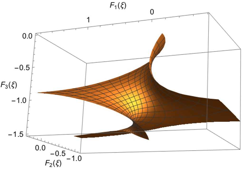
The Laguerre equation.

3D numerical display of the Enneper-Weierstrass representation of the surface (3.23) describing the Laguerre equation, obtained by computing ξ0 = 1 + i and ξ = re, r ∈ [−3, 3], θ ∈ [0, 2π].

3.2. Solutions of the linear problem and soliton surfaces associated with orthogonal polynomials

We summarize our results in the form of tables, giving the explicit form of surfaces and LP elements. Each table is made of five parts: the meromorphic functions η (3.4) and χ (3.5), the components of the potential matrix 𝒰 (2.16), the components of the wavefunction Ψ defined by (2.36) and (2.37), the components of the surface F ∈ 𝔼3 (2.13), and the components of the surface F˜𝔰𝔲(2) (2.19).

In each case, we consider in the table the parameter λ ∈ ℂ\{0} of the LP (2.15), the parameters {νk : k = 1, 2,...,n} of the specific ODE, and four arbitrary integration constants c1 ∈ ℂ\{0}, c2, k1, k2 ∈ ℂ. To keep the expressions compact, in what follows, we use the notation z* to designate the complex conjugate of z. We identify the special functions appearing in the formulas at the bottom of each table, accompanied by the notations and the constraints, in certain cases. For example, for the Jacobi equation, a restriction on the domain of the parametrization is necessary in order to integrate the functions η and χ, to find the components of the surface and to ensure the convergence of the infinite series. This restriction arises from the chosen representation of the functions appearing in the integrands of the Enneper-Weierstrass formula (2.13)

DJacobi={ξ:|ξ|<1and|ξ+1|<2|α|}.(3.25)

Each table is accompanied by a numerical 3D representation of a selected surface obtained by fixing the parameters of the classical ODE considered, the parameter of the LP and the integration constants. To keep the expressions in the captions compact, we use the notation Fk0, k = 1, 2, 3 to specify that the parameters and constants have fixed values.

Fig. 2:

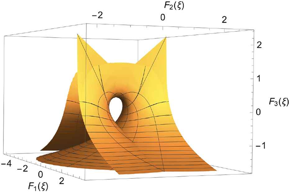
The Legendre equation. 3D numerical display of the Enneper-Weierstrass representation of the surface describing the Legendre equation, obtained by computing ξ0=12+i, ξ = re, where r ∈ [−8, 8], θ ∈ [0, 6π]. For fixed parameters and constants α = 1, c1 = 1, c2 = 0, k1 = 1, k2 = −1, λ = −2, we obtain

F10=12Re(z|ξ0ξ).F20=12Im([log(1+z)log(1z)z]ξ0ξ),F30=12Re(log(1z2)|ξ0ξ).

Fig. 3:

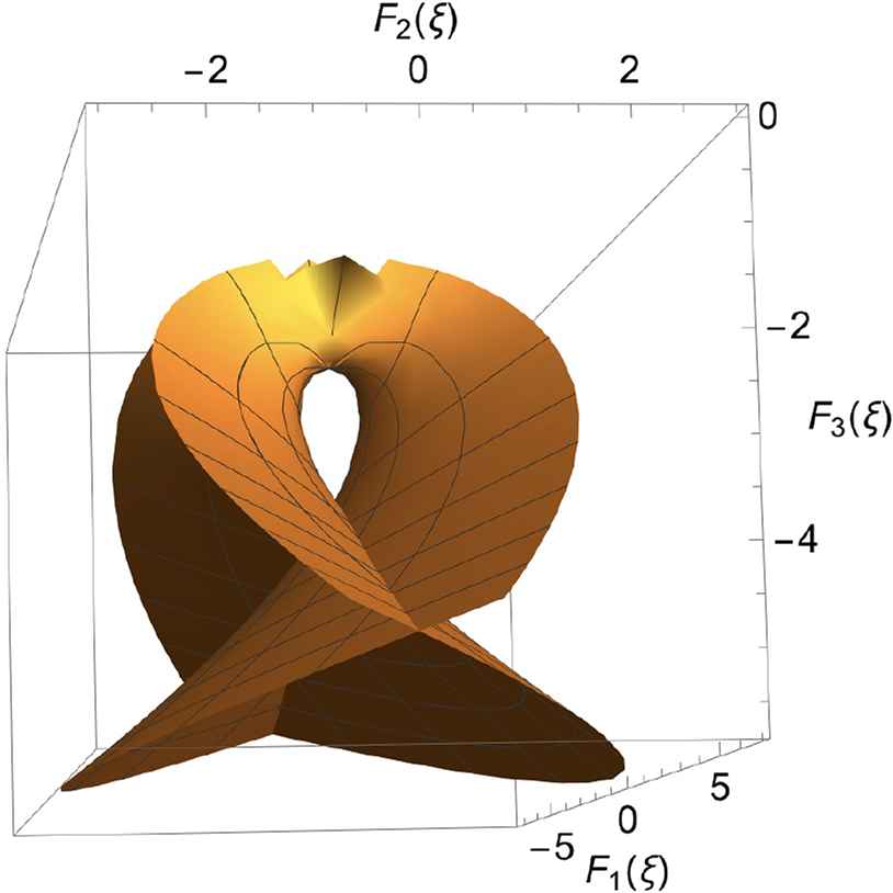
The Legendre associated equation. 3D numerical display of the Enneper-Weierstrass representation of the surface describing the Legendre associated equation, obtained by computing ξ0 = −1 − i, ξ = re, where r ∈ [−5, 5], θ ∈ [0, 2π]. For fixed parameters and constants α = 1, m = 1, c1 = 1, c2 = 0, k1 = 1, k2 = −1, λ=12, we obtain

F10=12Re([152(log(1+z)log(1z))+4z]ξ0ξ),F20=12Im([172(log(1+z)log(1z))4z]ξ0ξ),F30=2Re([log(z21)]ξ0ξ).

Fig. 4:

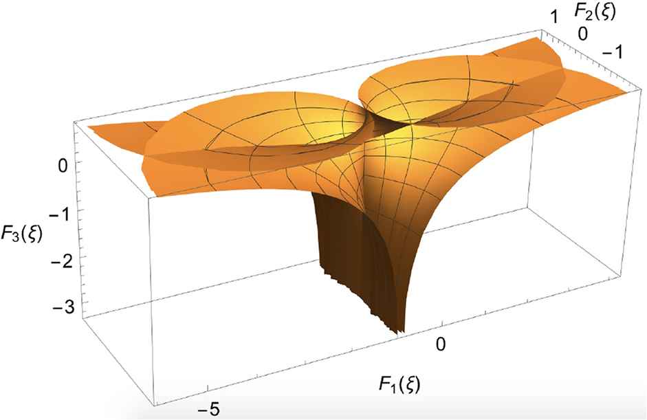
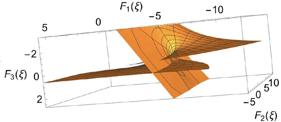
The Bessel equation.

3D numerical display of the Enneper-Weierstrass representation of the surface describing the Bessel equation, obtained by computing ξ0 = 1 and ξ = re, where r[1100,2], θ ∈ [0, 2π]. For fixed parameters and constants p = 0, c1 = 1, c2 = 0, k1 = 1, k2 = 1, λ = −1/2, we obtain

F10=12Re[(log(z)z44)|ξ0ξ],F20=12Im[(log(z)+z44)|ξ0ξ],F30=12Re[z2|ξ0ξ].

Fig. 5:

The Chebyshev equation. 3D numerical display of the Enneper-Weierstrass representation of the surface describing the Chebyshev equation, obtained by computing ξ0 = 1, ξ = re, where r ∈ [−10, 10], θ ∈ [0, 2π]. For fixed parameters and constants n = 1, c1 = 1, c2 = 0, k1 = 1, k2 = 1, λ = −1, we obtain

F10=12Re([arcsin(z)13arcsin3(z)]ξ0ξ),F10=12Im([arcsin(z)+13arcsin3(z)]ξ0ξ),F30=12Re(arcsin2(z)|ξ0ξ).

Fig. 6:

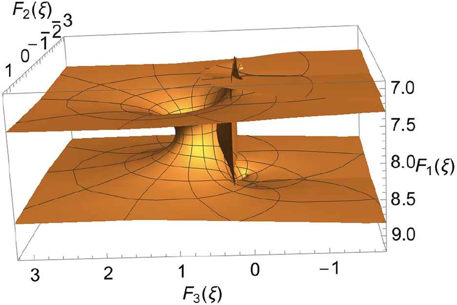
The Laguerre associated equation.

3D numerical display of the Enneper-Weierstrass representation of the surface describing the Laguerre associated equation, obtained by computing ξ0 = 3 + 3i, ξ = x + iy, where x ∈ [−3, 3], y[164,3]. For fixed parameters and constants α = 1, n = 2, c1 = 1, c2 = 0, k1 = 1, k2 = 1, λ = 1, we obtain

F10=12Re([32Ei(z)12ez(1z+1z2)+ez(z+5+6z+2z2)]ξ0ξ),F20=12Im([52Ei(z)12ez(1z+1z2)ez(z+5+6z+2z2)]ξ0ξ),F30=Re([log(z)2z1z2]ξ0ξ).

Fig. 7:

The Hermite equation.

3D numerical display of the Enneper-Weierstrass representation of the surface describing the Hermite equation, obtained by computing ξ0 = 1 + 3i and ξ = x + iy, x ∈ [−2, 2], y ∈ [−2, 2]. For fixed parameters and constants n = 1, c1 = 1, c2 = 0, k1=1π, k2 = 1, λ=π, we obtain

F10=12Reξ0ξ(1erf2(z))ez2dz,F20=12Imξ0ξ(1+erf2(z))ez2dz,F30=1πRe(z2F22(1,1;32,2;z2)|ξ0ξ).

Fig. 8:

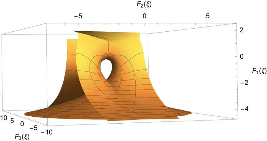
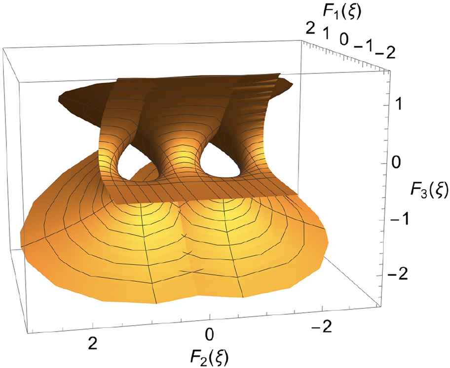
The Gegenbauer equation.

3D numerical display of the Enneper-Weierstrass representation of the surface describing the Gegenbauer equation, obtained by computing ξ0 = 0, ξ = re, r[1100,10], θ ∈ [0, 2π]. For fixed parameters and constants α=12, n = 1, c1 = 1, c2 = 0, k1 = 1, k2 = −1, λ = 1, we obtain

F10=Re([log((1z)(1+z))]ξ0ξ),F20=Im([log(1+z)log(1z)z]ξ0ξ),F30=Re(z|ξ0ξ).

Fig. 9:

The Jacobi equation.

3D numerical display of the Enneper-Weierstrass representation of the surface describing the Jacobi equation, obtained by computing ξ0 = 0, ξ = x + iy, x[1+1100,0], y[0,11100]. For fixed parameters and constants α = 1, β = 2, n = 1, c1 = 1, c2 = 0, k1 = 1, k2 = 1, λ = −1, we obtain

F10=132Re([(6z(z+1)+4(z1)(z+1)2+3(log(z+1)log(z1)))259(94z4+5z3172z255z+321z48log(z1)+2254)]ξ0ξ),F20=132Im([(6z(z+1)+4(z1)(z+1)2+3(log(z+1)log(z1)))+259(94z4+5z3172z255z+321z48log(z1)+2254)]ξ0ξ),F30=512Re([2z1+3log(z1)]ξ0ξ).

4. Concluding remarks

In this paper, we have shown the connection between the linear problem, the reduction of the GW equations to an ODE and the immersion functions of 2D-surfaces associated with classical special functions ODEs (SFODE) describing orthogonal polynomials. These links are summarized by the following diagram

Fig. 10:

Representation of the relations between the GW equations, the ODE associated with selected special functions and their immersion functions of 2D-surfaces.

This approach allows us to visualize the image of the surfaces arising from specific orthogonal polynomials, reflecting their behavior. The images were generated with Mathematica using the <monospace>ParametricPlot3d</monospace> command (no specific package). In order to reduce the calculation time, the primitive integrals of each component of the surface were used instead of the integral representation of the Enneper-Weierstrass formula.

The existence of SL(2, ℂ)-valued gauge transformations allowed the reduction of the LP to a second-order ODE, which can very often be explicitly integrated in terms of special functions. We showed that the simplification of the LP associated with the moving frame by successive gauge transformations allows the introduction of the arbitrary holomorphic functions η and χ of the Enneper-Weierstrass representation into the problem. This link between the immersion function and the LP was used to determine the second-order linear ODE arising from CMC-λ surfaces. At this point, the ODE representation of the LP could have been associated with any second-order linear ODE. We chose classical ODEs describing orthogonal polynomials, using the degree of freedom corresponding to the fact that the holomorphic functions η and χ are arbitrary. The explicit expressions for the potential matrices and the wavefunction solutions of the LP have been found. This fact enabled the construction of soliton surfaces defined using the Weierstrass or the Sym-Tafel formulas for immersion.

We have formulated easily verifiable conditions which ensure the visualization of surfaces describing special functions. This result can assist future studies of 2D-surfaces with the so-called Askey-scheme of hypergeometric orthogonal polynomials and their q-analogue of this scheme, which can lead to the description of more diverse types of surfaces than those studied in this paper. This task will be considered in a future work.

A new class of minimal surfaces describing orthogonal polynomials has been constructed. These surfaces must now be characterized to enable a clear description of their behavior in order to establish the links between their intrinsic properties and the orthogonal polynomials considered to construct them. The fundamental forms need to be determined, together with the genus and the zeros. We found that the orthogonality interval of the polynomials sometimes describes a curve on the surface. The link between this fundamental interval and the surfaces needs to be studied.

Acknowledgments

V.C. has been partially supported by the Natural Science and Engineering Research Council of Canada (NSERC) and by the Fonds de Recherche du Québec-Nature et Technologies (FRQNT). A.M.G. has been partially supported by the Natural Science and Engineering Research Council of Canada (NSERC) and would like to thank A. Doliwa (University of Warmia and Mazury) and D. Levi (University of Roma Tre) for helpful discussions on this topic.

References

[5]D.J. Gross, T. Piran, and S. Weinberg, Two dimensional quantum gravity and random surfaces, World Scientific Singapore, 1992.
[7]Z.-C. Ou-Yang, J.-X. Liu, Y.-Z. Xie, and X. Yu-Zhang, Geometric methods in the elastic theory of membranes in liquid crystal phases, World Scientific, 1999.
[10]A. Sommerfeld, Lectures on theoretical physics, Academic Press, Vol. 1-3, 1964.
[14]F. Olver, Asymptotics and special functions, Academic press, New York, 1974.
[15]M. Abramowitz and I.A. Segun, Handbook of Mathematical Functions, Dover, New York, 1965.
[16]E.D. Rainville, Special functions, The MacMillan Company, New York, 1960.
[17]A. Doliwa and A.M. Grundland. Minimal surfaces in the soliton surface approach, arXiv ID: 1511.02173 (2015)
[19]K. Weierstrass, Fortsetzung der untersuchung über die minimalflachen, Mathematische Werke, Vol. 3, 1866, pp. 219-248.
[20]A. Enneper, Analytisch-geometrische untersuchungen nachr, Königl. Gesell. Wissensch. Georg–Augusts-Univ. Göttingen, Vol. 12, 1868, pp. 258-277.
[27] Wolfram Research, Exponential integral, accessed in november 2018. URL: http://functions.wolfram.com/06.35.02.0001.01
Journal
Journal of Nonlinear Mathematical Physics
Volume-Issue
27 - 4
Pages
529 - 549
Publication Date
2020/09/04
ISSN (Online)
1776-0852
ISSN (Print)
1402-9251
DOI
10.1080/14029251.2020.1819599How to use a DOI?
Copyright
© 2020 The Authors. Published by Atlantis Press and Taylor & Francis
Open Access
This is an open access article distributed under the CC BY-NC 4.0 license (http://creativecommons.org/licenses/by-nc/4.0/).

Cite this article

TY  - JOUR
AU  - Vincent Chalifour
AU  - Alfred Michel Grundland
PY  - 2020
DA  - 2020/09/04
TI  - Minimal surfaces associated with orthogonal polynomials
JO  - Journal of Nonlinear Mathematical Physics
SP  - 529
EP  - 549
VL  - 27
IS  - 4
SN  - 1776-0852
UR  - https://doi.org/10.1080/14029251.2020.1819599
DO  - 10.1080/14029251.2020.1819599
ID  - Chalifour2020
ER  -