
Germinal Center Optimization Algorithm
- DOI
- 10.2991/ijcis.2018.25905179How to use a DOI?
- Keywords
- Germinal Center; Artificial Immune Systems; Evolutionary Optimization
- Abstract
Artificial immune systems are metaheuristic algorithms that mimic the adaptive capabilities of the immune system of vertebrates. Since the 1990s, they have become one of the main branches of computer intelligence. However, there are still many competitive processes in the biological phenomena that can bring new advances for many applications. The Germinal Center reaction is one of these competitive processes that had not been fully modeled until now, and that was the inspiration to design the novel optimization algorithm that we present in this work. Our proposal implements a competitive-based nonuniform distribution to select particles to be mutated, which can be interpreted as an implementation of temporal leadership in population-based metaheuristics. We model the dark-zone and light-zone of the Germinal Center and their competitive processes like clonal expansion, T-cell binding and life signal decay. We also propose the combination of this selection method with the use of one Differential Evolution-based strategy to substitute the somatic hypermutation process. To show the performance, we include a benchmark with the comparison of our approach versus some of the state-of-the-art bio-inspired optimization algorithms. We show that the proposal has a statistically significant improvement over the other algorithms for low dimensionality problems.
- Copyright
- © 2018, the Authors. Published by Atlantis Press.
- Open Access
- This is an open access article under the CC BY-NC license (http://creativecommons.org/licences/by-nc/4.0/).
1. Introduction
Optimization plays a big roll in nowadays scientific research and industrial developments, but for many of these applications is difficult to formalize a mathematical model to optimize, for this reason, metaheuristic algorithms have become a suitable solution. Metaheuristic optimization algorithms offer good solutions in affordable time for complex problems. A big branch of these algorithms is the so-called bio-inspired algorithms, and they are computational metaphors of biological phenomena that express great capabilities of adaptation.
An essential type of bio-inspired technique is the one based on the adaptive response of vertebrates immune system,1 which is the base for designing the Artificial Immune System (AIS) algorithms.2 As we will show in section 2, AIS algorithms have become a very active research field, with many successful algorithms which solve optimization, combinatorial and machine learning problems.
In the biological phenomena of adaptive immune response, we can find the Germinal Center Reaction. The Germinal Centers (GCs) are compartments within secondary lymphoid organs with two histologically distinctive zones: the light zone and the dark zone.3
As it is mentioned in Ref. 3, GCs are sites where B lymphocytes (B-cells) have clonal expansion, somatic hypermutation, and affinity-based selection. These processes result in the production of high-affinity antibodies.
GC presents non-deterministic competitive processes that offer a good metaphor for an artificial immune system algorithm. These features were first noticed in Ref. 4, where the authors proposed a novel algorithm called GC-AIS (Germinal Center Artificial Immune System), to solve the set-cover problem obtaining a good result. After that, they present a solution for the population explosion in the work detailed in Ref. 5.
In GC-AIS, the authors use the communication between GC as a parallelization property, although every GC mutates its candidate solutions with standard bit mutation in parallel. This approach is useful not only for the combinatorial problem but also for optimization and even for multi-modal optimization as well.
Nevertheless, the property mentioned above is just one of the many features of GCs. We believe that the recent research in GC, published in Refs. 6, 7, 8, 9, 10 recent researches imply that the affinity maturation problem is guided strongly by the affinity-based selection in the light zone and the clonal and mutation processes in the dark zone. Then, the dynamic of the light and dark zone is an important process in the Germinal Center operation that has to be implemented to take full advantage of all the functions of this process as we show in next sections.
In this paper, we present a novel optimization algorithm based on the recent research in GCs. This algorithm is a metaheuristic to model a competitive-based non-uniform distribution for candidate solutions selection.
The distribution is modeled following the GC reaction and offers a way to include temporal leadership for selecting particles in population-based metaheuristics. We apply this concept in a hybrid Differential Evolution algorithm, and we show statistically that we can get better or equal results in different optimization problems.
This paper is organized as follows, in section 2, we offer a short review of the Artificial Immune Systems fundamentals and main algorithms. In section 3, we describe the Differential Evolution and Particle Swarm Optimization algorithms. Next, in section 4 we discuss the Germinal Center Reaction. In section 5, we present the novel algorithm, in section 6, the experiments, and results are shown. Finally in section 7, we offer our conclusions.
2. Artificial Immune Systems
The vertebrate immune system can recognize, destroy and remember almost an unlimited number of Antigens (Ag) (foreign non-self objects in the body).11 These capabilities make the immune system a source of inspiration for many intelligent algorithms denominated Artificial Immune Systems (AIS).
There are two kinds of adaptive response in the natural immune system,1 the humoral immunity and the cellular immunity. The first one is formed by molecules present in blood and mucous secretions that have the name of Antibodies (Ab). The Ab is produced when a Lymphocyte B differentiates into a plasmatic cell. The Ab recognizes the Ag, neutralizes it and marks it for destruction. The effectiveness of the Ab to bound to an Ag is called affinty. The affinity of the Ab is changed in clonal proliferation and mutation of the B-cells through a process called Somatic Hypermutation.
The humoral immune response protects the body from Ag in blood but is not capable of detecting Ag inside cells, for example, the viruses and phagocytosed microbes. In this case, the body uses the cellular immunity, based on lymphocytes T (T-cells). There are two kinds of T cells, on the one hand, the cytotoxic T-cell, that directly destroys infected cells and the helper T-cell that activates infected macrophages to kill inner microbes among other functions. Summarising, in the adaptive response we have extracellular protection with the humoral immunity (produced by B-cells) and intracellular protection with cellular immunity (thanks to T-cells). For a more in-depth introduction to immunity review Ref. 1.
Many AIS algorithms are based on different parts of the processes expressed above. In Fig. 1, we present a taxonomy of the principal AIS algorithms families based on Refs. 2 and 11. These algorithms have gained popularity, and they have many successful applications like computer security, optimization, data mining and anomaly detection.2
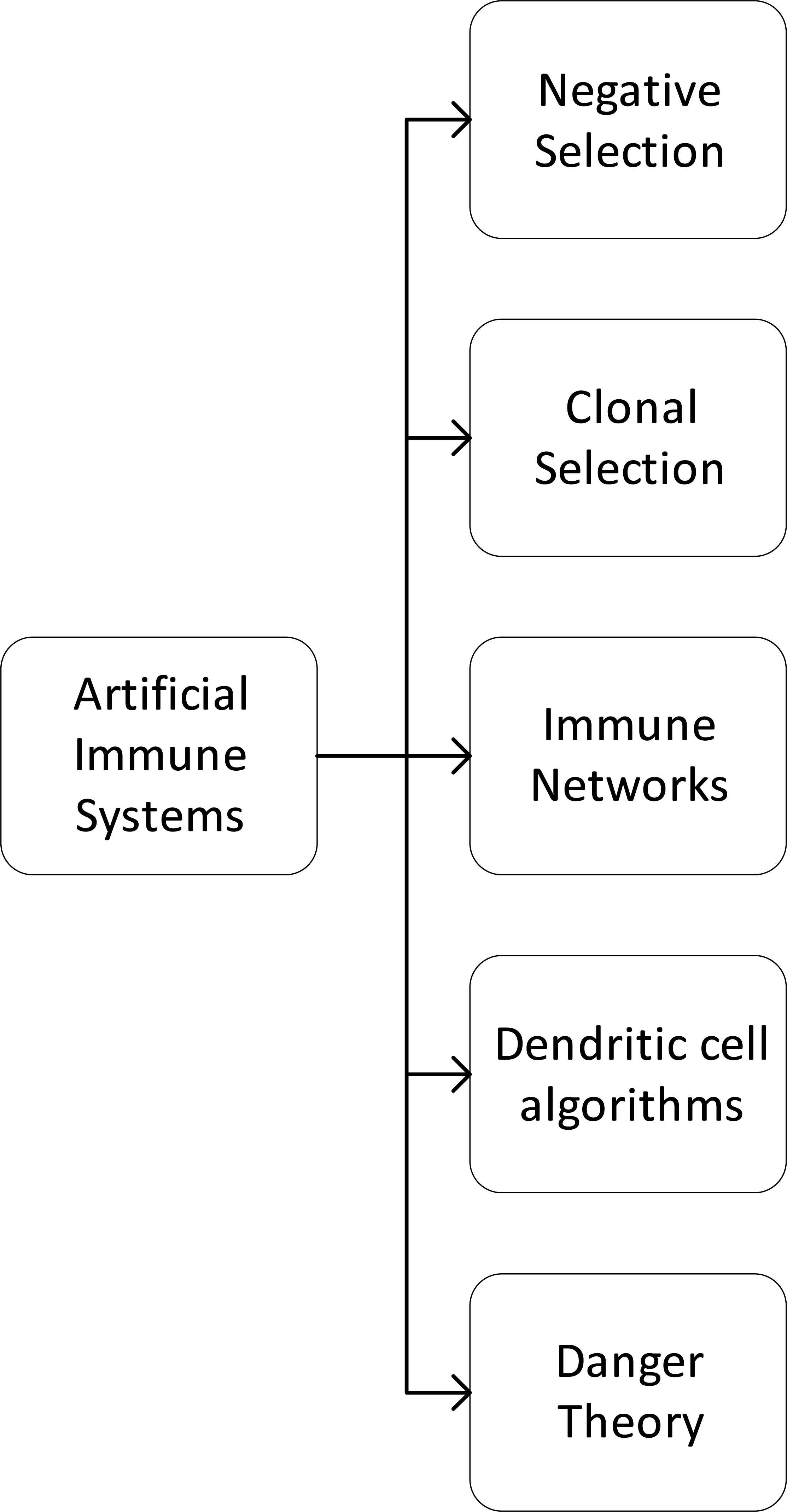
Principal techniques in AIS
Negative Selection Algorithm (NSA) is based on the self/nonself immunological paradigm model, where the ongoing selection of cells is performed just like it has been observed in the preparation of naive T-cells, which mature with the positive and negative selection. Clonal Selection Algorithms (CLONALG) are inspired by clonal selection theory, which is based on the proliferation of B and T-cells, that mutate with somatic hypermutation and differentiate in plasmatic cells or memory B-cell with different lifespan. Artificial Immune Networks (AIN) are based on the work of Jerne12, where he explains that immune cells interact not only with Ag, but also with the previous Ab, and this could trigger clonal selection. Dendritic Cell Algorithms (DCA) are a family of algorithms based in Danger Theory proposed by Matzinger13, that suggest that the adaptive immune system reacts to danger signals and dendritic cells are part of the innate immune system that responds to some specific danger signals. Many other algorithms have been proposed based on Danger theory.13
3. Metaheuristic Algorithms
In this section, we briefly explain five successful evolutionary algorithms. Evolutionary optimization algorithms14 are metaheuristic algorithms based on evolutionary competence, and they have been proven to be a good solution for multivariate problems.
3.1. Differential Evolution
Differential Evolution15 (DE) is a successful optimization algorithm for multivariate functions. DE is a population-based metaheuristic. Then, the algorithm propose a population of N Candidate Solutions, also known as particles. Each particle compete with the others to get the best evaluation of the objective function. The particles are initialized randomly in the search space, then for each particle pi in the population a mutant
A random recombination is done with (2) for every dimension j ∈ {1, ⋯ ,D} of the problem, where r ∼ U[0,1], is a continuously uniform random number, CR is the Cross-Ratio.
Finally, the mutant is selected only if it has a better performance in the objective function f(·) using (3). Where the mutant that outperforms the actual particle, takes the place of the particle.
DE is memory efficient because only the best solution is kept, and in time, because it performs only a few basic operations. This particular implementation is denoted DE/rand/1, for the random selection for the mutation process.
3.2. Particle Swarm Optimization
Particle Swarm Optimization16 (PSO) is based on collective intelligence, where every particle competes among others but is also influenced by the performance of other particles. There are two influences in the particle dynamics, first we are influenced by the leader pl (the particle with the best solution) and in the second instance by the best past positions of the particle
We add this velocity to the correspondent particle position with (5)
Finally, we have to keep track of the best solution then we can calculate the leader index l with
3.3. Gravitational Search Algorithm
Gravitational Search Algorithm17 (GSA) is based on the Newtonian gravitational theory and movement laws, where the gravitational force is an analogy of the attraction of the best particles. The main difference between GSA and PSO is that in GSA every particle influences the other particles, and particles with better fitness have a greater attraction. For every particle we calculate a fitness mi with (7). Then, the fitness is normalized in (8) to get Mi.
We calculate the force that a particle k apply to the i-th particle with (9), where G is the gravitational constant. Using the second law of Newton, we calculate an acceleration in (10), where r ∼ U[0,1]. Finally, using ai we calculate the velocity and position of each particle in (11–12), where r ∼ U[0,1].
To ensure the convergence of GSA, the Gravity constant G has to decrease every iteration, for this we use an exponential decay in (13), where α is the decay parameter, t is a discrete time counter, and tmax is the maximum number of iterations.
The basic idea behind GSA is that the performance of each particle Mi is a force of attraction in the particles interaction. GSA is computationally more expensive than DE or PSO, because it models a fully connected topology of interactions, although there are already variations that fix this problem, we use this version because it is an example of a fully connected topology.
3.4. Genetic Algorithm
The Genetic Algorithm18 (GA) is one of the earliest and most used evolutionary algorithms. The GA models the phenotype inheritances through and elitist pairing and random mutations. GA initializes a random population of phenotypes that iterate three different processes listed below.
Selection: We calculate a fitness for each phenotype with (14), where f(·) is the objective function. Then, we pair them using Roulette Selection.14 With this selection the phenotypes with the best performance tend to mate.
Crossover: For each pair of phenotypes, we merge their information using blending technique in (15), where β is the blending factor, C1 and C2 are the produced children, x1 and x2 are the phenotype parents. Later, we substitute the parents with the children.
Mutation: We perform random mutation in the phenotypes population, we calculate s ∼ U[1,N] and w ∼ U[1,d] and mutate with (16).
GA proposes a performance-based paring to inheriting the information and ensure explorations through a mutation process.
3.5. Artificial Bee Colony
Artificial Bee Colony19 (ABC) is an evolutionary algorithm based on the different behaviors of bees. ABC simulates the search of optimal food source with three different behaviors listed below.
Forager bees: Every forager bee is associated to ax specific location,14 and moves around by randomly selecting another forager bee, this process is similar to DE/rand/1 algorithm.
Onlooker bees: The Onlooker bees change its position using Roulette Selection of the forager bees, this process is like GA algorithm.
Scout bees: When a forager bee stagnates we reset it with a scout bee. The scout bee looks randomly in the search space until it finds a better position for the forager bee.
We can see the ABC algorithm as a way to merge DE and GA.
3.6. Leadership in Evolutionary Optimization
A critical factor in Evolutionary Optimization is the balance between exploration and exploitation. Exploration refers to the ability of a particle to search in a wide neighborhood; this is important to avoid local minima, but the particle can move away from the global minimum. On the other hand, exploitation refers to the ability to approach infinitesimally to the minimum; this is important to get a better solution, but the particle can get stuck in a local minimum. Leadership is a way to select other particles based on some feature to generate new candidate solutions.
On the right hand, PSO calculates all new candidate solutions with the best particle, this high leadership benefits the exploitation of the search space but limits explorations. On the left hand, DE in its variation DE/rand/1 uniformly selects three particles to generate a new candidate. This variation has no leadership, this property benefits explorations but limits exploitation.
In GSA a particle influence in other particles depends on its performance, but the algorithm is slower than PSO and DE because it calculates for a pair of particles. GA offers another solution, using Roulette selection14 based on particles fitness, and we pair the particles to procreate new solutions. Although, the way GA mutates and generates new solutions has not the best exploration. Finally, ABC uses two swarms with different typologies and different behaviors. In the forager bees we found a leaderless exploration (like in DE/rand/1), and in the onlooker bees, we have a performance-based selection like in GA.
In the next section, we present biological phenomenon called Germinal Center Reaction. Based on this phenomenon, we propose a new algorithm that could merge different leaderships based on a competitive scheme. The algorithm simulates the B-cells that compete to get the best Abs. The multiplicity distribution of the B-cells is a non-uniform distribution that changes through time adapting the leadership and producing delayed leadership as we show in the next sections.
4. Germinal Center reaction
As we already established, the immune system can respond to foreign substances Ag by producing Ab that bind to Ag with extremely high affinity. This unexpected high affinity is the result of a phenomenon called Affinity Maturation (AM). The AM takes place in structures known as GCs, that were first described in 1884 by Walther Flemming20 as distinct microanatomical regions in secondary lymphoid organs.
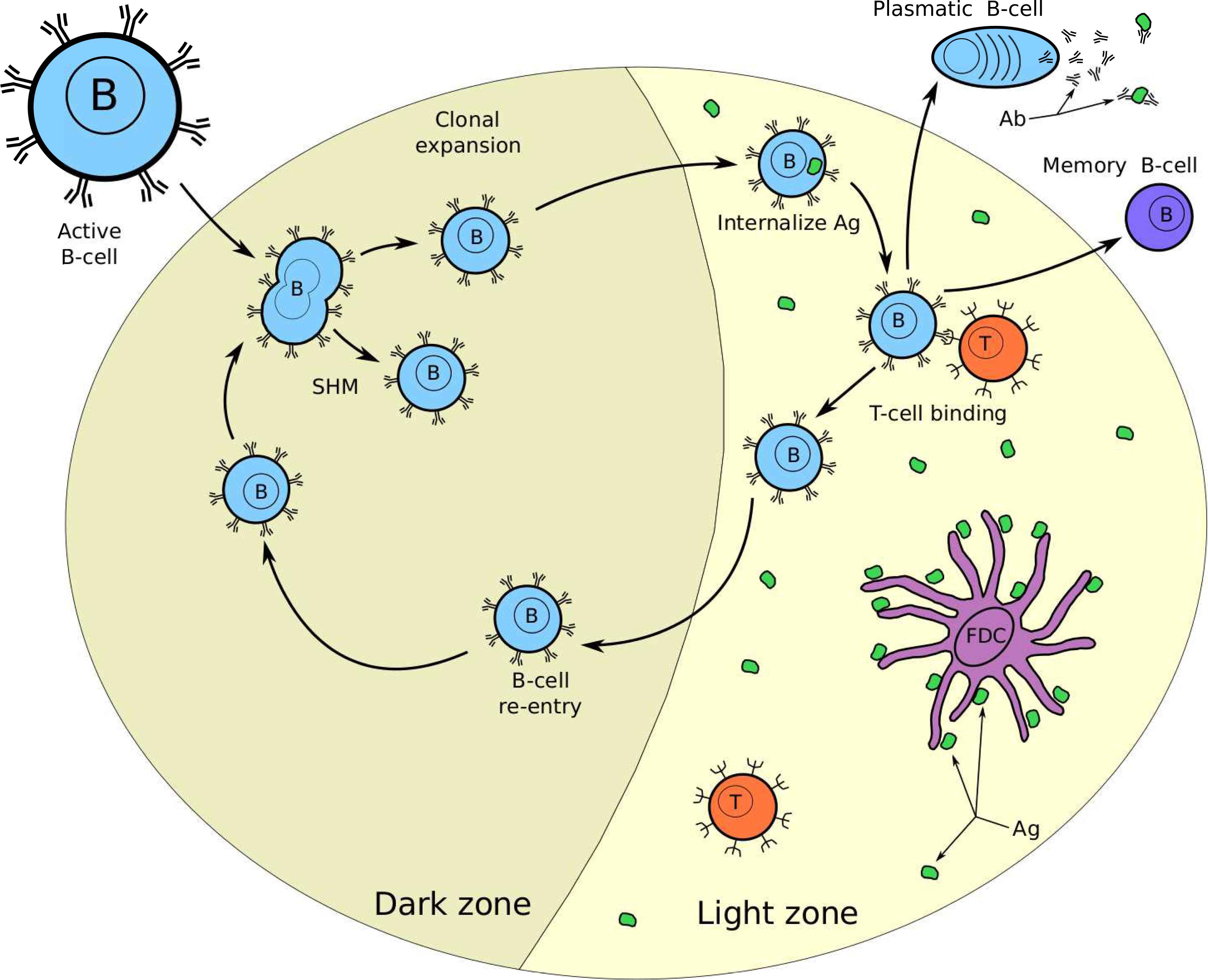
Recent research3 indicated that the GCs are sites for B-cell clonal expansion, somatic hypermutation (SHM), and affinity-based selection. This process is called GC reaction and is the principal responsible for AM.3 The GC is divided into two zones, the Dark Zone (DZ), where clonal expansion and somatic hypermutation take place and the Light Zone (LZ), where competition for Ag internalization and Helper T-cell binding takes place.
In Fig. 2, we show a GC reaction diagram. In the rest of this section, we will explain briefly the GC reaction, in order to set a suitable computational analogy.
Germinal Center reaction. The GC forms in the presence of Ag and is divided in two zones. In the Dark zone, the B-cell proliferate through clonal expansion and SMH. In the Light zone the B-cells compete for Ag, and helper T-cell binding.
4.1. GC formation
GCs develop after the activation of B-cells in the secondary lymphoid nodes, the B-cells migrate into the follicular system where they begin monoclonal expansion in the environment of follicular dendritic cells (FDC).9 The activated B-cells differ from the surrounding naive B-cell (inactive) in many ways. The naive cells rarely divide, but GC B-cells are among the fastest dividing mammalian cells with a cell-cycle time at 6-12 hours.3 GC FDCs act like an Ag reservoir that supports AM. Also, FDC play an important role in GC polarization in LZ/DZ.3
4.2. Clonal expansion and Somatic hypermutation
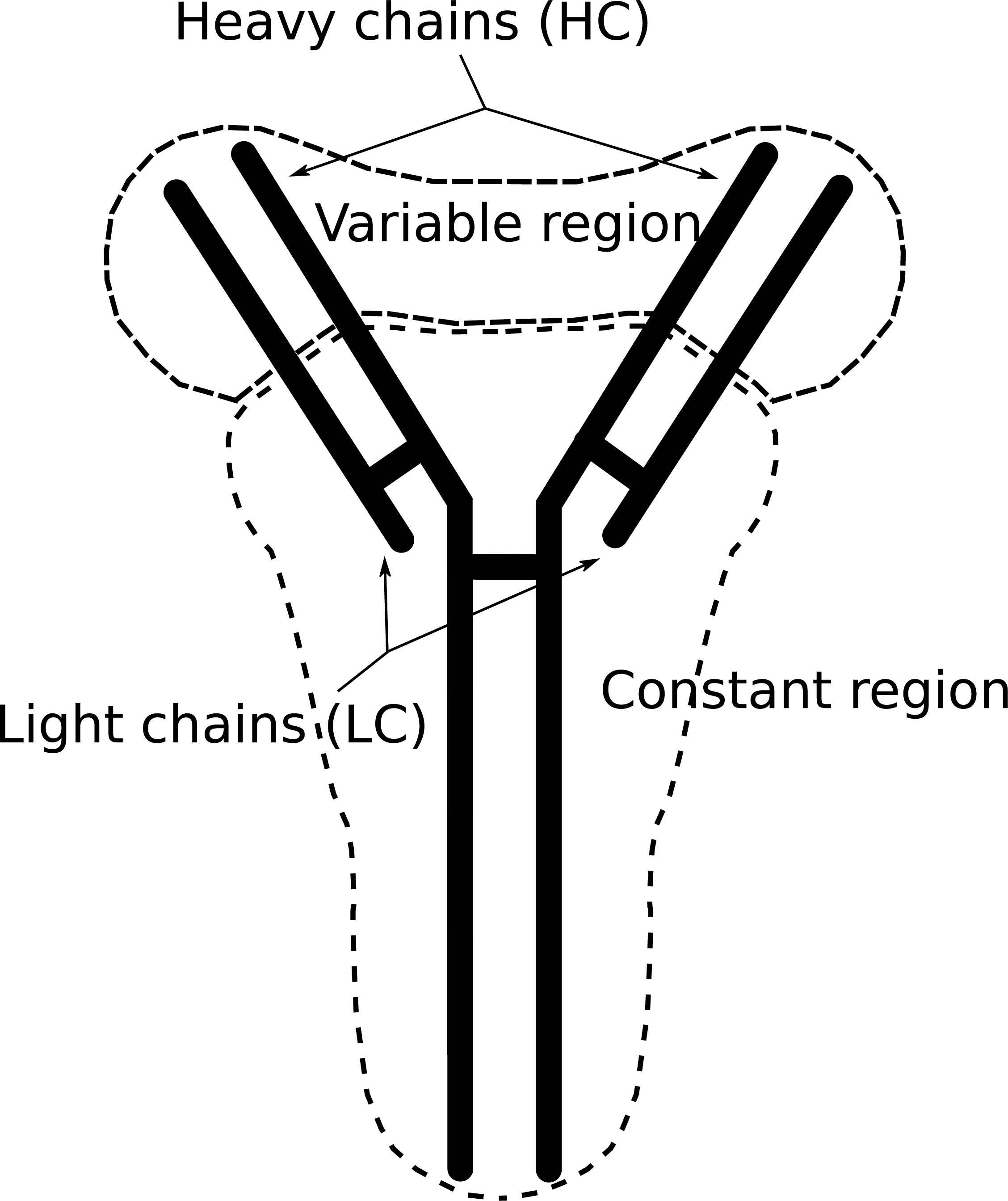
Inside the GC in the DZ, activated B-cells start proliferating. In this process, mutation takes place, some of these mutations affect the affinity of the Ab. In Fig 3, we present an Ab scheme, the Ab is divided into two zones, the constant region, and the variable region, there are also two kinds of chains, the heavy chain, and the light chain. The variable region plays a big roll in Ag binding, and for this reason, it is important to define the affinity Ab-Ag. The adaptation in AM in GC means to change the variable region to get higher affinity. The process that changes this region is called somatic hypermutation (SHM) as mentioned in Refs. 21, 22 and 23.
Antibody. The anybodies are shaped proteins produced by plasmatic B-cells and their function is to neutralize Ag. The variable zone mutates through SHM leading to high diversity
A theory that explains how SHM is capable of producing high specialized Ab is called VDJ renomination theory. This theory solved a puzzle for immunologists for many decades and supported the idea of high diversity Ab. For the constant part, there is another process called Class Switch Recombination (CSR), this process changes the B cell production of Immunoglobulin (Ig) Isotope from one to another.
4.3. Antigen Internalization
After the proliferation in the DZ, the centrocytes (B-cell with a cleaved nucleus) have initiated apoptosis, and they have a finite lifetime.9 They need to be rescued from apoptosis by the interaction with Ag and T-helper cells. Then, B cells migrate to the LZ and compete for antigen in FDC.
4.4. Helper T-cell binding
After antigen internalization, the B-cell needs to present Ag to a T-helper cell to get a life signal. An important fact is that this two-step process of finding Ag and finding a T-helper cell, constitutes an affinity-based selection process, because the B-cell could not internalize Ag with low affinity then, the B cells with the best affinity can get the life signal from the T-helper cell. These two competitive steps reward B-cells with the best affinity with more lives, and they are very similar to a Darwinian Selection process.
The model proposed in Ref. 6, presents two probabilities, first the probability of a B cell internalizing Ag, and the probability of a B-cell succeeding in receiving T-cell help. These probabilities work with a measure of the affinity binding based on each peptide (part of the antigen recognized by the B-cell). For a better understanding of the T-helper cell, the reader can review Ref. 24.
4.5. B-cell recycling or output
The Ag internalization and T-helper cell binding are competitive processes that happen both inside and outside GC, the main difference between them is what happens with the B cell after T-helper cell binding. We have three paths the B-cell can follow.
The first one is re-entry to the DZ and proliferates again. In this path, is the principal path, because it allows getting better affinity through generations and competition, and it is also the reason why we get high-affinity antibodies from the GC reaction.
The second one is to get out of the GC and differentiate in a plasmatic cell. In this path, will liberate antibodies in the blood helping the humoral immune response.
The third and final path is to get out of the GC and become a memory B-cell. Memory B-cells have a long lifespan and work like Ag-specific antibodies reservoir. They can even get into new GCs and compete again.
5. Germinal Center Optimization algorithm
In this section, we will present our proposal of an AIS algorithm based on GC that we call Germinal Center Optimization (GCO) algorithm. First, let us set in the next list the competitive features that make GCs a suitable framework for an AIS algorithm:
- 1.
SHM and clonal expansion (sec. 4.2): Ensure antibodies diversity which allows a good coverage (and exploration) of the solution search area.
- 2.
- 3.
Re-entry in DZ (sec. 4.5): Iterative affinity improvement, which ensures a high precision in the obtained solution.
- 4.
Memory B-cell (sec. 4.5): Communication with others GCs and long-term memory of the solution.
An essential part of the GC philosophy is that a B-cell that has better affinity can extend its lifespan. Therefore it could proliferate and mutate with higher probability; consequently, this also increments the likelihood for the T-helper cell binding process. When we develop a bio-inspired algorithm, it is crucial to design a useful abstraction, to get a low computational and memory cost. In Table 1, we present the computational metaphor between a GC and an optimization problem. The Antigen could be related to the objective function f : ℝn → ℝn that we want to optimize. The Ab and B-cells represent the candidates solutions Bi ∈ ℝn and the affinity is the objective function evaluation, f (Bi). Finally, the T-help cell binding is an increment of the life-signal of the B-cell.
| Germinal Center | Optimization problem |
|---|---|
| Antigen | Objective function |
| Antibody and B-cell | Candidate solution |
| Affinity | Objective function evaluation |
| T-help cell binding | Incrementation of life-signal |
Computational metaphor
The primary task of the proposal is to dynamically model a non-uniform probability distribution based on B-cells multiplicity (clones of the B-cell), and the Life signal (probability of B-cell to duplicate or die). In comparison with Refs. 4 and 5, our proposal implements the DZ and LZ like processes in the optimization algorithm, as we show in Fig. 4.
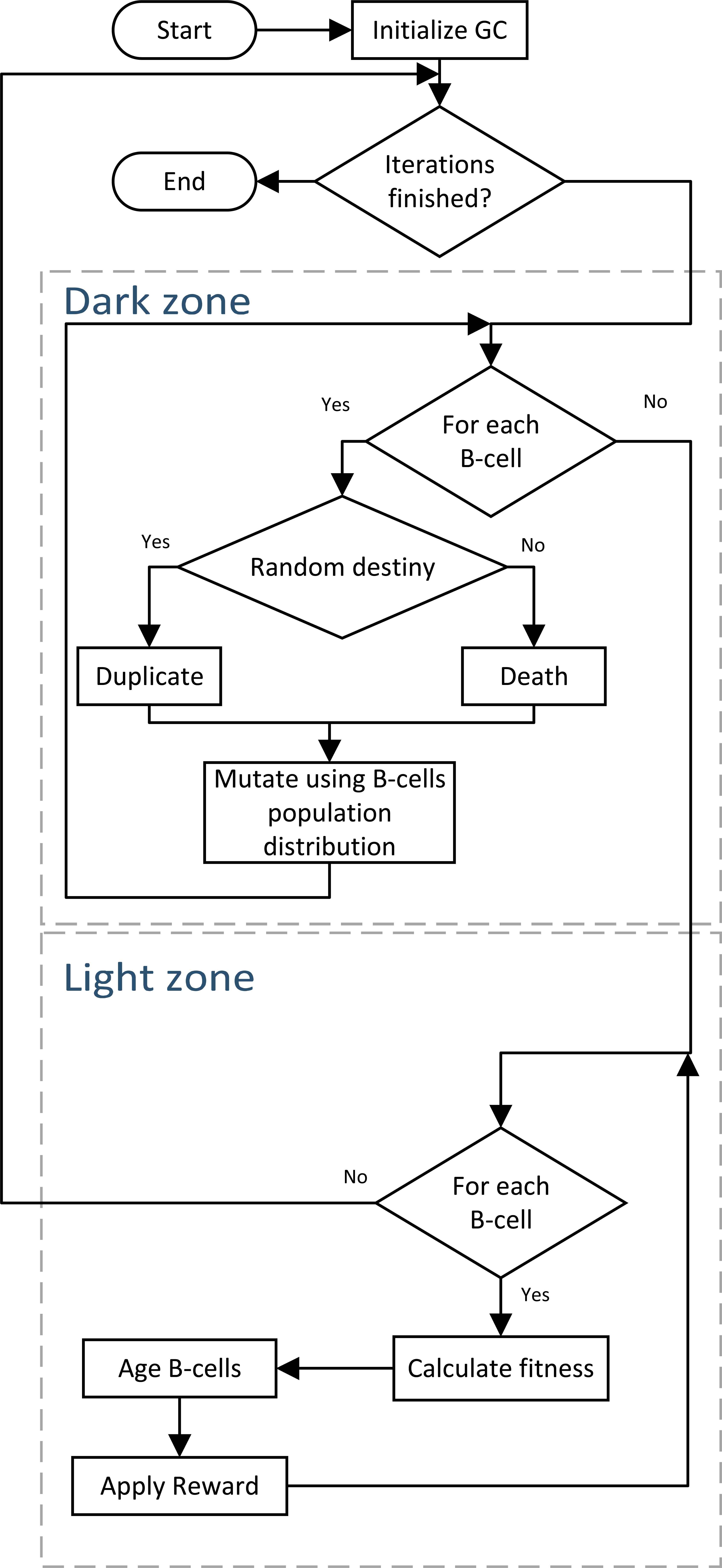
GCO algorithm flowchart
5.1. GCO scheme
In Fig. 4, we show the algorithm flowchart, and in the Alg. 2 and 1, we offer complete pseudocode of the proposed algorithm. In this section, we describe the GCO scheme.
First, we initialize a population of B-cells with cardinality N, every B-cell Bi stores a candidate solution of dimension d that is initialized randomly in the search space. We also set a cell counter in every B-cell to one. Every Bi has a life-signal 𝔏 that is initially set to 70; this initial number means that initially, the cell has 70% chances to duplicate and 30% to die. The 𝔏 changes through time, and depends on the B-cell performance.
After initialization, we start every iteration of the algorithm with the Dark-zone process. First, for every Bi we calculate a random number rl ∼ U[0,100] and compare it to the life signal of Bi, that way we decide to duplicate or kill the B-cell. Duplicate the B-cell, means to add one to the cells counter of the B-cell and the GC. Kill the B-cell, means to rest one to the cells counter, this process emulates clonal expansion (sec. 4.2). Then, the life signal 𝔏 controls a simulated population of the Germinal Center.
We continue with a mutation process very similar to the DE mutation. The idea is to emulate somatic hypermutation, described in section 4.2, with the way DE mutate cells, this is computationally efficient, because biologically most of the mutations do not affect the affinity3. To store all mutations (candidate solutions) and to random evaluate them is memory expensive and it causes slow convergence, as we have experimented in early versions of this proposal.
The principal difference with DE mutation is that DE uses a uniform distribution to select the particles for mutation, this process denies the idea of leadership. This has shown to be useful in the PSO algorithm. Instead, we model a discrete non-uniform distribution 𝒞 (cell population distribution), where the B-cell with more copies is more likely to influence the mutant.
The distribution 𝒞 implements an adaptive leadership with delay, based on the B-cell performance. After mutation, we start the Light-zone process, where an aging process is emulated with the 𝔏 decay. Then, we calculate the B-cell fitness, using the same formula as in GSA17, this allows rewarding the B-cells with different Life-signals with the idea that the best B-cell does not age.
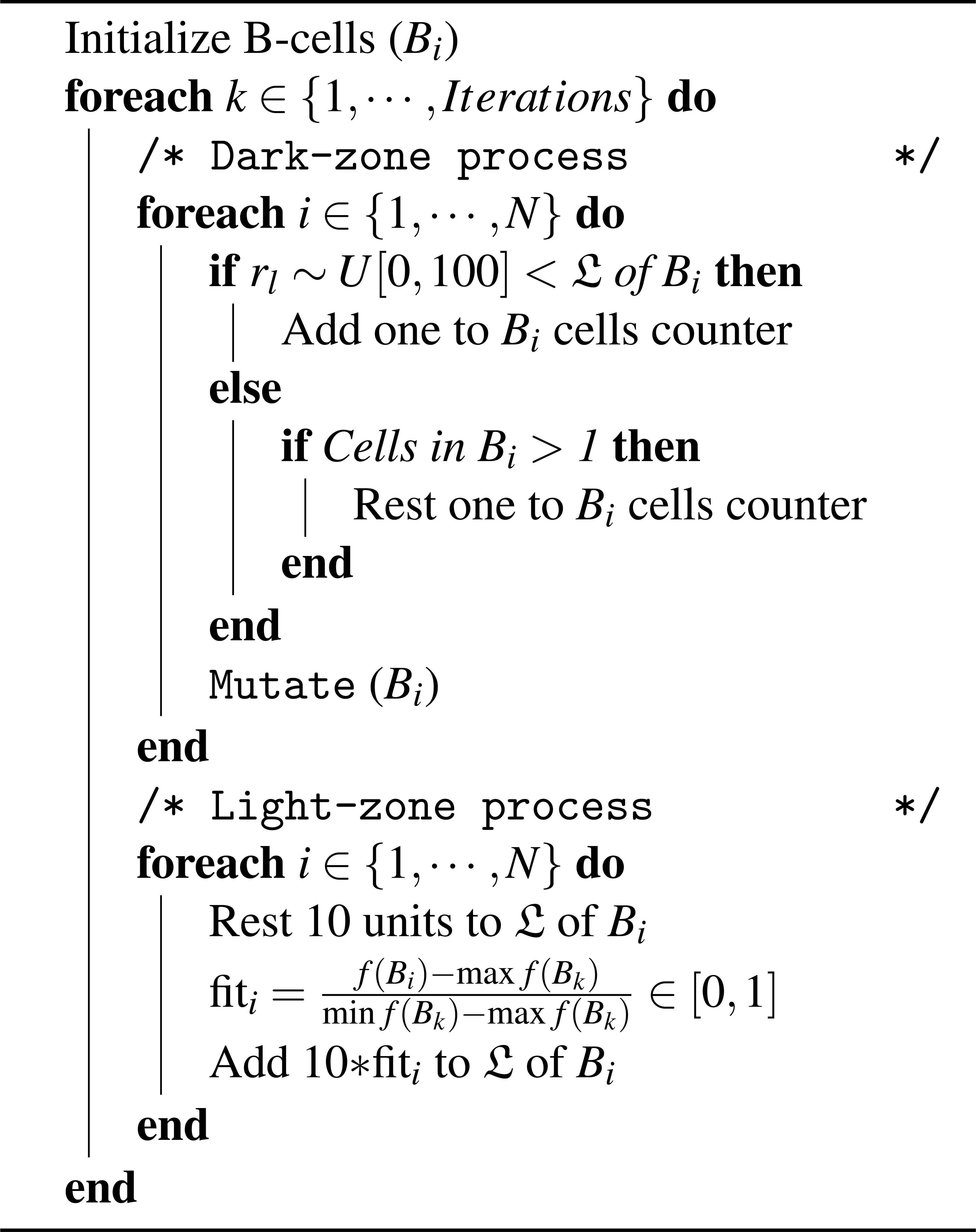
GCO algorithm
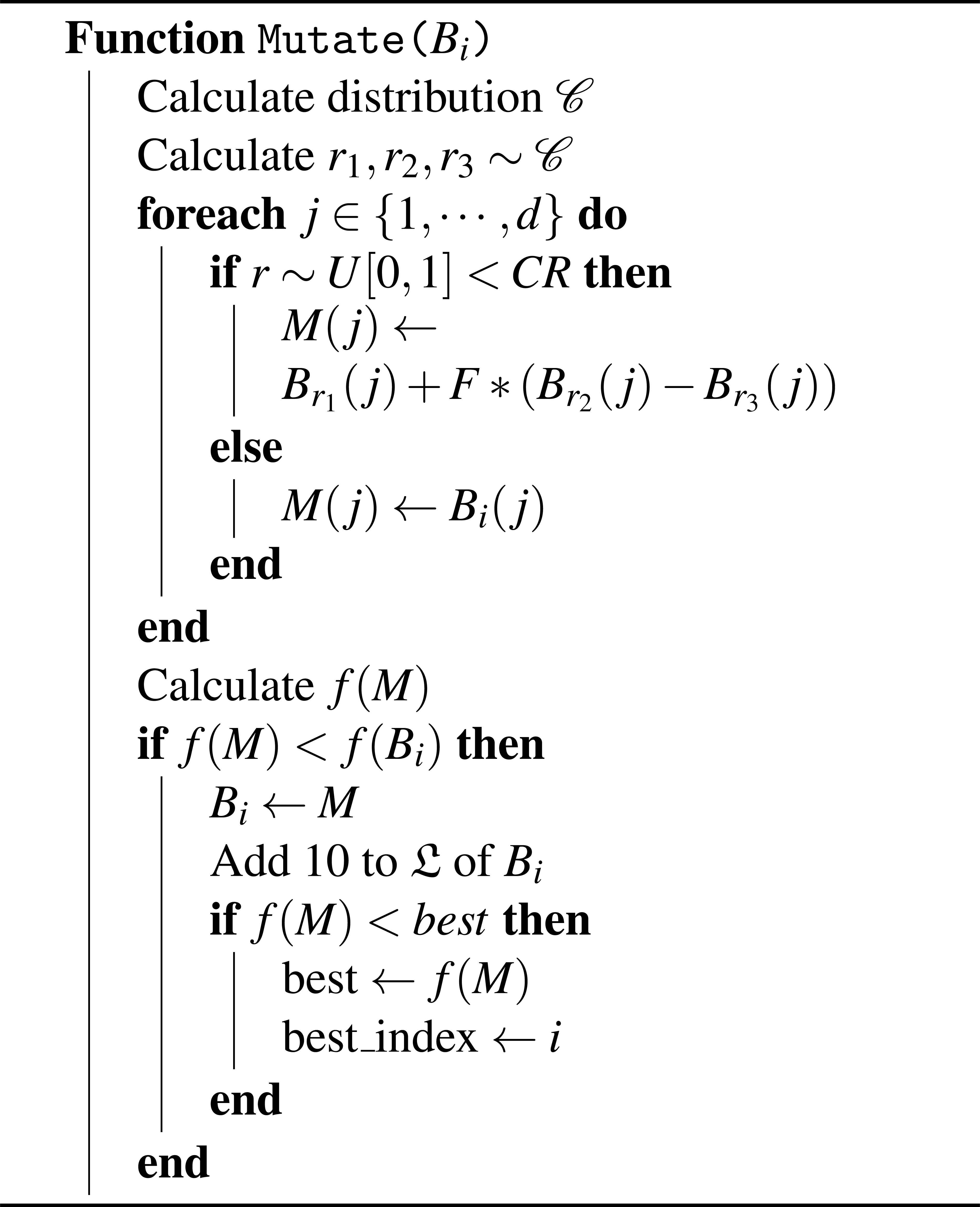
Mutate function
6. Experiments and Results
To show our proposal capabilities, we offer the following experimentation benchmark and nonparametric statistical proof. We present 18 test functions in the next subsection with their respective Search Space (SS) bounds. The functions f1 to f7 are convex and soft functions, from f8 to f12 are functions with many local minima. f13 is a plate-shaped function and f14 and f15 have a valley-shaped form. Moreover, the others are miscellaneous functions. The variable d is the dimension.
We ran 30 test for every function and every algorithm in low dimension (two dimensions) and high dimension (30 dimensions). These tests were carried out in a Xeon CPU E31225 with 3.10 GHz and 8 Gb of RAM. For all the algorithms in the low dimension test, we used 500 iterations with 40 particles, and for the high dimension test, we used 1000 iterations and 40 particles.
6.1. Benchmark functions
- •
Sphere with SS [−5.12,5.12]d
- •
Sum of Squares with SS [–5.12, 5.12]d
- •
Rotated Hyperellipsoid with SS [–65.53,65.53]d
- •
Perm 0, d, β with SS [–d,d]d
- •
Sum of different powers with SS [–1,1]d
- •
Trid with SS [–d2,d2]d
- •
Bochachevsky with SS [−15,15]d
- •
Ackley with SS [−32.76,32.76]d
- •
Griewank with SS [−600,600]d
- •
Levy with SS [−10,10]d
- •
Rastrigin with SS [−5.12,5.12]d
- •
Schwefel with SS[−500,500]d
- •
Zakharov with SS [−5,10]d
- •
Dixon-Price with SS [−10,10]d
- •
Rosenbrock with SS [−5,10]d
- •
Michalewicz with SS [0,π]d
- •
Perm d, β with SS [−d,d]d
- •
Styblinski-Tang with SS [−5,5]d
For the GCO and DE algorithms we used CR = 0.7 and F = 1.25, for PSO c1 = c2 = 1.49618 and w = 0.729844. For GSA, the parameters are set with G0 = 100 and α = 20, for GA we used a mutation rate of 20%, and finally, for ABC we used Pf = N/2 and L = Nn/2.
6.2. Low dimension tests
In Table 2, we show the results of low dimension tests. Every element in the table is the form μ ± σ, where μ is the mean value achieved by the algorithms in 30 tests, and σ is the standard deviation. Note that in most cases the GCO algorithm overcomes the other algorithms. In the other cases the GCO still has a good performance. We are also able to see that the standard deviation of GCO tends to be smaller in most of the benchmark functions.
| f | GCO | DE | PSO | GSA | GA | ABC |
|---|---|---|---|---|---|---|
| f1 | 1.53e-55 ± 4.58e-55 | 3.43e-52 ± 1.41e-51 | 2.82e-21 ± 1.53e-20 | 3.08e-18 ± 3.42e-18 | 3.27e-02 ± 5.68e-03 | 5.01e-55 ± 2.61e-54 |
| f2 | 1.29e-53 ± 7.06e-53 | 4.95e-53 ± 1.19e-52 | 3.48e-23 ± 1.80e-22 | 2.61e-18 ± 2.81e-18 | 1.99e-02 ± 2.93e-03 | 5.76e-54 ± 2.63e-53 |
| f3 | 1.89e-53 ± 5.77e-53 | 1.17e-50 ± 2.86e-50 | 1.60e-22 ± 7.70e-22 | 2.74e-18 ± 2.40e-18 | 1.33e-04 ± 3.23e-05 | 9.44e-51 ± 5.15e-50 |
| f4 | 3.18e-22 ± 1.62e-21 | 1.35e-24 ± 7.39e-24 | 5.14e-24 ± 1.25e-23 | 3.08e-03 ± 1.18e-02 | 3.92e-04 ± 1.62e-04 | 4.38e-03 ± 4.78e-03 |
| f5 | 2.41e-66 ± 1.04e-65 | 3.70e-63 ± 1.71e-62 | 4.87e-27 ± 2.67e-26 | 1.29e-02 ± 1.48e-02 | 4.89e-01 ± 6.12e-02 | 1.32e-46 ± 5.02e-46 |
| f6 | −2.00e+00 ± 0.00e+00 | −2.00e+00 ± 0.00e+00 | −2.00e+00 ± 0.00e+00 | −2.00e+00 ± 1.97e-05 | - | −2.00e+00 ± 0.00e+00 |
| f7 | 0.00e+00 ± 0.00e+00 | 0.00e+00 ± 0.00e+00 | 0.00e+00 ± 0.00e+00 | 0.00e+00 ± 0.00e+00 | 2.47e-03 ± 4.82e-04 | 0.00e+00 ± 0.00e+00 |
| f8 | 4.44e-16 ± 2.00e-31 | 4.44e-16 ± 2.00e-31 | 2.20e-12 ± 6.10e-12 | 3.73e-09 ± 1.77e-09 | 4.38e-02 ± 3.28e-04 | 5.62e-16 ± 6.48e-16 |
| f9 | 2.21e-03 ± 3.44e-03 | 4.93e-04 ± 1.87e-03 | 2.60e-03 ± 3.52e-03 | 6.35e-02 ± 5.96e-02 | 9.74e-03 ± 2.15e-03 | 4.47e-05 ± 2.10e-04 |
| f10 | 1.92e-26 ± 8.75e-42 | 1.92e-26 ± 8.75e-42 | 3.57e-24 ± 1.85e-23 | 7.54e-19 ± 1.15e-18 | 2.24e-03 ± 6.32e-04 | 1.98e-26 ± 3.65e-27 |
| f11 | 0.00e+00 ± 0.00e+00 | 0.00e+00 ± 0.00e+00 | 0.00e+00 ± 0.00e+00 | 1.39e-01 ± 2.01e-01 | 1.78e-02 ± 2.23e-03 | 2.36e-16 ± 1.29e-15 |
| f12 | 1.33e+01 ± 3.44e+01 | 1.35e+00 ± 7.40e+00 | 5.13e+01 ± 6.73e+01 | 1.49e+02 ± 1.04e+02 | 8.07e-04 ± 6.61e-05 | - |
| f13 | 6.91e-51 ± 1.73e-50 | 6.03e-48 ± 2.08e-47 | 4.21e-25 ± 1.64e-24 | 2.65e-18 ± 2.92e-18 | 7.18e-05 ± 3.34e-05 | 2.30e-33 ± 1.26e-32 |
| f14 | 3.86e-32 ± 4.26e-33 | 6.60e-28 ± 3.57e-27 | 1.00e-21 ± 4.50e-21 | 1.89e-17 ± 3.01e-17 | 2.01e-05 ± 1.01e-05 | 2.80e-06 ± 3.79e-06 |
| f15 | 1.44e-26 ± 7.25e-26 | 4.94e-24 ± 1.68e-23 | 2.71e-15 ± 1.23e-14 | 5.08e-02 ± 5.99e-02 | 8.81e-04 ± 5.09e-04 | 1.37e-02 ± 2.22e-02 |
| f16 | −1.80e+00 ± 6.77e-16 | −1.80e+00 ± 6.77e-16 | −1.72e+00 ± 2.44e-01 | −1.16e+00 ± 2.58e-01 | - | −1.80e+00 ± 6.77e-16 |
| f17 | 7.10e-03 ± 3.89e-02 | 0.00e+00 ± 0.00e+00 | 9.41e-24 ± 3.45e-23 | 9.40e-05 ± 1.54e-04 | 1.67e-02 ± 1.24e-03 | 4.27e-04 ± 5.74e-04 |
| f18 | −7.83e+01 ± 2.89e-14 | −7.83e+01 ± 2.89e-14 | −7.83e+01 ± 2.89e-14 | −7.83e+01 ± 2.89e-14 | - | −7.83e+01 ± 2.89e-14 |
Low dimension results (Mean ± Standard deviation)
In Table 3, the run-time of the low dimension tests is shown. GCO is slower than DE and PSO, this is due to the linear complexity of evaluating the nonuniform probability distribution. Note that GCO is faster than GSA, GA and ABC. PSO is the fastest algorithm in the tests. Finally, we claim that GCO is a good option for low dimension problems.
| f | GCO | DE | PSO | GSA | GA | ABC |
|---|---|---|---|---|---|---|
| f1 | 1.0200e-02 | 7.6667e-03 | 3.1333e-03 | 8.7433e-02 | 8.7433e-02 | 8.7433e-02 |
| f2 | 1.0000e-02 | 7.6667e-03 | 2.9000e-03 | 8.8200e-02 | 8.8200e-02 | 8.8200e-02 |
| f3 | 9.8667e-03 | 7.8333e-03 | 2.8000e-03 | 8.8167e-02 | 8.8167e-02 | 8.8167e-02 |
| f4 | 1.1033e-02 | 9.3333e-03 | 4.6000e-03 | 8.9300e-02 | 8.9300e-02 | 8.9300e-02 |
| f5 | 9.5667e-03 | 8.0000e-03 | 3.0667e-03 | 1.1170e-01 | 1.1170e-01 | 1.1170e-01 |
| f6 | 1.1533e-02 | 9.6667e-03 | 5.4667e-03 | 9.0033e-02 | 9.0033e-02 | 9.0033e-02 |
| f7 | 9.6000e-03 | 7.5667e-03 | 3.4000e-03 | 8.8667e-02 | 8.8667e-02 | 8.8667e-02 |
| f8 | 1.0467e-02 | 8.5667e-03 | 4.1333e-03 | 8.8633e-02 | 8.8633e-02 | 8.8633e-02 |
| f9 | 1.0333e-02 | 8.2667e-03 | 4.0000e-03 | 8.8500e-02 | 8.8500e-02 | 8.8500e-02 |
| f10 | 1.4300e-02 | 1.2467e-02 | 7.8667e-03 | 9.2067e-02 | 9.2067e-02 | 9.2067e-02 |
| f11 | 9.6333e-03 | 7.8333e-03 | 3.2667e-03 | 8.8700e-02 | 8.8700e-02 | 8.8700e-02 |
| f12 | 1.0200e-02 | 8.3333e-03 | 4.0667e-03 | 9.2400e-02 | 9.2400e-02 | 9.2400e-02 |
| f13 | 1.1600e-02 | 9.7667e-03 | 5.1000e-03 | 9.1133e-02 | 9.1133e-02 | 9.1133e-02 |
| f14 | 1.1467e-02 | 9.6667e-03 | 5.0333e-03 | 9.0900e-02 | 9.0900e-02 | 9.0900e-02 |
| f15 | 1.1733e-02 | 9.6667e-03 | 5.0333e-03 | 9.2033e-02 | 9.2033e-02 | 9.2033e-02 |
| f16 | 1.3167e-02 | 1.1400e-02 | 6.5667e-03 | 8.9433e-02 | 8.9433e-02 | 8.9433e-02 |
| f17 | 1.1300e-02 | 9.4000e-03 | 4.7333e-03 | 8.9000e-02 | 8.9000e-02 | 8.9000e-02 |
| f18 | 1.1067e-02 | 9.3667e-03 | 4.9000e-03 | 9.0900e-02 | 9.0900e-02 | 9.0900e-02 |
Low dimension mean time (seconds)
6.3. High dimension tests
In Table 4, we show the results for high dimension tests. GCO does not get better results than GA, GSA, and ABC in high dimension problems, but it has more similar performance than DE and PSO. It is important to note, that the algorithms that did not perform well in low dimension, in high dimensions they perform better. The opposite happens to GCO, DE, and PSO, they perform well in low dimension, but not in high dimension tests.
| f | GCO | DE | PSO | GSA | GA | ABC |
|---|---|---|---|---|---|---|
| f1 | 4.01e+01 ± 1.37e+01 | 1.46e+02 ± 1.30e+01 | 4.37e+00 ± 9.95e+00 | 7.48e-16 ± 3.35e-16 | 5.74e-03 ± 5.72e-04 | 7.14e-08 ± 1.09e-07 |
| f2 | 5.01e+02 ± 1.52e+02 | 1.53e+03 ± 1.64e+02 | 9.52e+01 ± 1.30e+02 | 6.98e-06 ± 2.47e-05 | 3.43e-04 ± 5.08e-05 | 9.16e-07 ± 1.10e-06 |
| f3 | 8.29e+04 ± 2.76e+04 | 2.56e+05 ± 2.88e+04 | 2.58e+04 ± 2.74e+04 | 9.35e-03 ± 5.12e-02 | 2.17e-06 ± 2.22e-07 | 2.58e-04 ± 5.20e-04 |
| f4 | 1.61e+90 ± 6.18e+90 | 3.36e+91 ± 2.24e+91 | 5.02e+30 ± 2.75e+31 | 7.06e+25 ± 3.84e+26 | 2.27e-92 ± 1.59e-92 | 3.91e+02 ± 2.72e+02 |
| f5 | 2.80e-01 ± 3.22e-01 | 1.90e+00 ± 5.51e-01 | 2.11e-17 ± 9.55e-17 | 1.44e-08 ± 2.67e-08 | 2.86e-01 ± 1.06e-01 | 1.44e-12 ± 3.68e-12 |
| f6 | 6.67e+05 ± 3.55e+05 | 6.80e+05 ± 3.77e+05 | 3.09e+05 ± 2.86e+05 | 1.14e+05 ± 3.66e+04 | - | 1.12e+04 ± 5.31e+03 |
| f7 | 1.21e+03 ± 5.03e+02 | 3.56e+03 ± 4.14e+02 | 1.14e+02 ± 2.19e+02 | 2.82e-01 ± 5.04e-01 | 2.07e-04 ± 7.24e-05 | 3.27e-05 ± 3.11e-05 |
| f8 | 1.92e+01 ± 8.51e-01 | 2.07e+01 ± 9.38e-02 | 1.77e+00 ± 4.35e+00 | 1.74e-08 ± 3.77e-09 | 4.16e-02 ± 1.38e-02 | 1.80e-02 ± 7.59e-03 |
| f9 | 1.34e+02 ± 5.13e+01 | 5.06e+02 ± 5.79e+01 | 1.21e+01 ± 3.11e+01 | 6.23e+00 ± 2.49e+00 | 1.54e-03 ± 5.37e-04 | 3.13e-04 ± 4.15e-04 |
| f10 | 8.56e+02 ± 3.18e+02 | 1.70e+03 ± 1.19e+02 | 2.19e+02 ± 9.08e+01 | 1.52e-01 ± 4.68e-01 | 3.11e-04 ± 1.05e-04 | 4.91e-06 ± 6.61e-06 |
| f11 | 2.37e+02 ± 4.69e+01 | 3.76e+02 ± 1.77e+01 | 1.22e+02 ± 3.51e+01 | 2.28e+01 ± 4.39e+00 | 1.72e-03 ± 5.76e-04 | 4.73e-02 ± 4.58e-02 |
| f12 | 3.28e+03 ± 3.49e+02 | 4.63e+03 ± 3.15e+02 | 3.80e+03 ± 7.62e+02 | 9.89e+03 ± 4.91e+02 | 6.34e-05 ± 2.11e-05 | −2.15e+06 ± 1.94e+06 |
| f13 | 6.08e+02 ± 6.57e+01 | 7.05e+02 ± 6.14e+01 | 5.02e+02 ± 2.31e+02 | 1.48e+02 ± 4.19e+01 | 1.37e-12 ± 6.01e-13 | 3.21e+02 ± 4.67e+01 |
| f14 | 2.98e+05 ± 1.38e+05 | 1.26e+06 ± 2.56e+05 | 8.51e+03 ± 3.50e+04 | 8.31e-01 ± 2.89e-01 | 3.49e-07 ± 1.27e-07 | 1.54e+00 ± 4.77e-01 |
| f15 | 1.96e+03 ± 6.57e+02 | 5.44e+03 ± 5.90e+02 | 1.03e+02 ± 2.38e+02 | 3.10e+01 ± 1.79e+01 | 9.47e-05 ± 3.42e-05 | 2.84e+01 ± 4.91e+00 |
| f16 | −1.70e+01 ± 1.71e+00 | −1.08e+01 ± 6.54e-01 | −1.96e+01 ± 1.90e+00 | −2.02e+01 ± 1.32e+00 | - | −2.79e+01 ± 3.20e-01 |
| f17 | 6.09e+85 ± 8.63e+85 | 5.02e+87 ± 4.25e+87 | 9.00e+80 ± 2.10e+81 | 8.11e+85 ± 1.09e+86 | 8.91e-90 ± 2.95e-90 | 3.13e+83 ± 8.63e+83 |
| f18 | −6.47e+02 ± 1.14e+02 | −3.18e+02 ± 6.76e+01 | −1.03e+03 ± 3.72e+01 | −7.97e+02 ± 5.24e+01 | - | −1.17e+03 ± 2.77e-01 |
High dimension results (Mean ± Standard deviation)
In Table 5 we show their run-time for high dimension test. The ”-” symbols denote that the algorithm did not converge to a solution. Note that PSO is still the fastest algorithm, while the other algorithms are close in run-time.
| f | GCO | DE | PSO | GSA | GA | ABC |
|---|---|---|---|---|---|---|
| f1 | 8.0300e-02 | 7.6767e-02 | 4.4067e-02 | 5.8220e-01 | 9.9364e-02 | 8.2733e-02 |
| f2 | 8.1867e-02 | 7.6600e-02 | 4.5000e-02 | 5.8243e-01 | 1.0118e-01 | 8.3700e-02 |
| f3 | 8.9500e-02 | 8.5200e-02 | 5.3900e-02 | 5.9170e-01 | 1.1000e-01 | 9.1600e-02 |
| f4 | 1.8294e+00 | 1.8356e+00 | 1.7860e+00 | 2.3136e+00 | 1.7911e+00 | 1.8050e+00 |
| f5 | 9.0400e-02 | 8.3567e-02 | 4.9767e-02 | 5.8833e-01 | 9.9000e-02 | 7.9700e-02 |
| f6 | 1.3840e-01 | 1.3487e-01 | 1.0347e-01 | 6.3973e-01 | 9.9000e-02 | 1.3380e-01 |
| f7 | 1.2903e-01 | 1.2517e-01 | 7.4567e-02 | 6.0120e-01 | 1.3382e-01 | 1.0910e-01 |
| f8 | 1.0740e-01 | 1.0080e-01 | 6.2967e-02 | 5.9373e-01 | 1.1091e-01 | 9.7033e-02 |
| f9 | 1.2347e-01 | 1.1903e-01 | 8.1000e-02 | 6.2167e-01 | 1.2045e-01 | 1.1720e-01 |
| f10 | 1.4553e-01 | 1.3870e-01 | 1.0407e-01 | 6.4247e-01 | 1.5673e-01 | 1.4017e-01 |
| f11 | 1.0450e-01 | 9.9000e-02 | 6.2000e-02 | 6.0013e-01 | 1.0945e-01 | 9.1233e-02 |
| f12 | 1.1493e-01 | 1.0963e-01 | 8.5000e-02 | 6.1250e-01 | 1.1591e-01 | 1.1093e-01 |
| f13 | 9.1100e-02 | 8.4033e-02 | 5.6267e-02 | 5.8867e-01 | 9.8545e-02 | 7.3733e-02 |
| f14 | 1.4660e-01 | 1.3750e-01 | 1.0430e-01 | 6.4217e-01 | 1.3655e-01 | 1.4060e-01 |
| f15 | 2.0573e-01 | 2.0210e-01 | 1.6440e-01 | 7.0447e-01 | 1.8227e-01 | 1.9483e-01 |
| f16 | 1.9483e-01 | 1.8317e-01 | 1.6037e-01 | 7.0757e-01 | 1.8227e-01 | 1.9777e-01 |
| f17 | 1.8314e+00 | 1.8441e+00 | 1.7777e+00 | 2.3071e+00 | 1.5835e+00 | 1.8095e+00 |
| f18 | 1.4827e-01 | 1.4227e-01 | 1.0213e-01 | 6.4737e-01 | 1.5835e+00 | 1.4020e-01 |
High dimension mean time (seconds)
6.4. Wilcoxon Rank-Sum test
To compare the algorithms, we used the Wilcoxon Rank-Sum test, which is a non-parametric test (no normal distribution is supposed). The Wilcoxon test proposes a Null hypothesis H0: The mean for two set of samples is the same. If the means are equal, this implies that the two process are statistically equivalent.
Wilcoxon test calculates the sign of all differences between samples, and it assigns a rank to each difference. Multiplying the rank by the sign, we find a mapping to a normal distribution. In this distribution, we measure the sparsity. If the Null hypothesis is accepted, the two processes are statistically equal, and in case of rejection, the two methods are significantly different.
In Table 6, we present the two tiled Wilcoxon tests of GCO and the other algorithms for all the functions on the benchmark with the p-values, calculated with (35), where k is the number of the arrangement of signs. The tests that reject the null hypothesis are denoted in bold letters. Based on Table 6, we can say that GCO is statistically different from DE, PSO, GSA, GA, and ABC for low dimension problems.
| f | GCO vs DE | GCO vs PSO | GCO vs GSA | GCO vs GA | GCO vs ABC |
|---|---|---|---|---|---|
| f1 | 2.4386e-09 | 3.0199e-11 | 3.0199e-11 | 3.0199e-11 | 5.6073e-05 |
| f2 | 1.8500e-08 | 3.0199e-11 | 3.0199e-11 | 3.0199e-11 | 1.5638e-02 |
| f3 | 8.9934e-11 | 3.0199e-11 | 3.0199e-11 | 3.0199e-11 | 1.2732e-02 |
| f4 | 3.0588e-02 | 4.1230e-08 | 1.9533e-11 | 1.9533e-11 | 1.9533e-11 |
| f5 | 4.9980e-09 | 3.0199e-11 | 3.0199e-11 | 3.0199e-11 | 4.9752e-11 |
| f6 | NaN | NaN | 1.2118e-12 | 1.6853e-14 | NaN |
| f7 | NaN | NaN | NaN | 1.2118e-12 | NaN |
| f8 | NaN | 5.8337e-09 | 1.2118e-12 | 1.2118e-12 | 3.3371e-01 |
| f9 | 3.1559e-02 | 1.0325e-01 | 2.1595e-10 | 4.0723e-10 | 6.6546e-03 |
| f10 | NaN | 1.9432e-09 | 1.2118e-12 | 1.2118e-12 | 1.6080e-01 |
| f11 | NaN | NaN | 8.8658e-07 | 1.2118e-12 | 3.3371e-01 |
| f12 | 4.5264e-02 | 2.7667e-02 | 7.7237e-10 | 3.8190e-05 | 6.4789e-12 |
| f13 | 2.0152e-08 | 3.0199e-11 | 3.0199e-11 | 3.0199e-11 | 3.0199e-11 |
| f14 | 2.3198e-01 | 1.9742e-11 | 4.0806e-12 | 4.0806e-12 | 4.0806e-12 |
| f15 | 8.8862e-10 | 3.0180e-11 | 3.0180e-11 | 3.0180e-11 | 3.0180e-11 |
| f16 | NaN | 8.1404e-02 | 1.2118e-12 | 1.6853e-14 | NaN |
| f17 | 3.3371e-01 | 1.1483e-03 | 4.5618e-11 | 4.5618e-11 | 4.5618e-11 |
| f18 | NaN | NaN | 1.2118e-12 | 1.6853e-14 | NaN |
p-values of the Wilcoxon Rank-Sum test for low dimension. (Bold letters indicates the null hypothesis rejection, NaN stands for Not a Number and means that the test did not converge)
7. Conclusion
The Germinal Center reaction is a mechanism to get high-affinity maturation to protect the body. This high affinity is achieved with multiple competitive processes. In the present paper, we have proposed a novel multivariate optimization technique based on the Germinal Centers. In comparison with the already proposed GC-AIS,4 which model multiple Germinal Centers, we implement for the first time an algorithm based on the Dark and Light zones and their competitive processes. The Germinal Center optimization algorithm, mimics the Dark-zone process like the clonal expansion with a multiplicity attribute, and Somatic hypermutation through a performance-based selection in a mutation process similar to Differential Evolution. In the Light-zone, the B-cells get a life signal proportional to their fitness in the same way as in GSA, and this is an analogy of the T-helper cell binding process.
The particle selection in mutation uses the Roulette Selection but with the multiplicity distribution of the B-cell. This distribution changes over time, allowing an adaptive leadership process. On the other hand, the multiplicity distribution is formed by the random method that depends on the life signal. This feature will enable a delay effect in the leadership of a B-cell that decays through generations. When a B-cell mutates and gets a better affinity the new cell substitute the older and renewing the life signal, this allows it to lose leadership. In our results, the GCO algorithm outperforms the other algorithms in most of the presented test function in low dimension, an in the high dimension we have the same performance like in DE and PSO. We consider this novel technique is a good competitor to the modern evolutionary algorithms and we recommend to use it when you do not have prior information of the objective function because its adaptive leadership will allow for a better average case performance.
Acknowledgements
The authors thank the support of CONACYT México, through Projects CB256769 and CB258068 (Project supported by Fondo Sectorial de Investigación para la Educación). This work was also supported by the DAAD (Deutscher Akademischer Austauschdienst) and the Alfons und Gertrud Kassel-Stiftung.
References
Cite this article
TY  - JOUR
AU  - Carlos Villaseñor
AU  - Nancy Arana-Daniel
AU  - Alma Y. Alanis
AU  - Carlos López-Franco
AU  - Esteban A. Hernandez-Vargas
PY  - 2018
DA  - 2018/11/01
TI  - Germinal Center Optimization Algorithm
JO  - International Journal of Computational Intelligence Systems
SP  - 13
EP  - 27
VL  - 12
IS  - 1
SN  - 1875-6883
UR  - https://doi.org/10.2991/ijcis.2018.25905179
DO  - 10.2991/ijcis.2018.25905179
ID  - Villaseñor2018
ER  -