
A Novel Interactive Fuzzy Programming Approach for Optimization of Allied Closed-Loop Supply Chains
- DOI
- 10.2991/ijcis.11.1.52How to use a DOI?
- Keywords
- Closed-Loop Supply Chain Optimization; Interactive Fuzzy Programming; Common Sources; Multi-Level Programming; Preferred Compromise Solution
- Abstract
In recent years, the relationship between companies and suppliers has changed with the continuous rise in environmental awareness and customer expectations. In order to fulfill customers’ needs, the actors in a Supply Chain (SC) network sometimes compete and sometimes cooperate with each other. In SC management, both competitive and collaborative strategies have become important and have required different points of view. In a collaborative environment, companies should strive for common targets with mutual relationship. After managers decided to share their resources, some positive effects have appeared on the companies and suppliers’ performance such as profitability, flexibility and efficiency. Consequently, many companies are willing to cooperate with each other in a SC network because of these reasons. On the other hand, Closed-Loop Supply Chain (CLSC) management has been attracting a growing interest because of increased environmental issues, government regulations and customer pressures. Based on this initiative, our paper presents a novel allied CLSC network design model with two different SCs including common suppliers and common collection centers. First, a decentralized multi-level Mixed-Integer Linear Programming (MILP) model that consists of two different levels of Decision Makers (DMs) is developed. The plants of common SCs comprise the upper-level DMs, common suppliers, common collection centers, and the logistics firm comprises the lower-level DMs. A novel Interactive Fuzzy Programming (IFP) approach using Fuzzy Analytic Hierarchy Process (AHP) is proposed to obtain a preferred compromise solution for the developed model. Through use of Fuzzy AHP in the proposed IFP approach, the DMs can identify the importance of the lower-level DMs. In order to validate the developed model and the proposed IFP approach, a numerical example is implemented. According to the obtained results, our proposed IFP method outperforms Sakawa and Nishizaki’s1 and Çalık et al.’s2 approach with respect to the satisfaction degrees of upper-level DMs for the developed CLSC model.
- Copyright
- © 2018, the Authors. Published by Atlantis Press.
- Open Access
- This is an open access article under the CC BY-NC license (http://creativecommons.org/licences/by-nc/4.0/).
1. Introduction
In today’s world, pressure of competition has considerably raised because of the increasing pressure of market competition and the globalization of the economy. Thus, SC and integrated logistics have gained importance among researchers and managers. A well-structured SC network enables firms to compete at a higher level in the market and helps them cope with increasing environmental concerns3. Companies need to improve their SCs to handle forward and reverse flows of goods more effectively. They should find new ways to be faster and to become more flexible in the market to satisfy customer expectations. To gain these advantages, many companies started to collaborate with each other. While doing so, many companies have focused on coordination (alliances) strategies4. One of the most important decisions in SC management is to design an SC network, which directly affects companies’ environmental and economic performance. In general, strategic decisions such as determining the locations of actors, the capacities of these actors, and the material flow between them are the most important questions in SC management5.
Many academicians and company managers have focused on Reverse Logistics (RL) and CLSC issues considering environmental, social, and economic factors. The vast number of publications which have been published in recent years is an evidence of this situation. The amount of publications in multi-objective decision making is fewer than on single objective studies. Handling real-world problems with multi-objective functions is more valuable than with single objective ones6. Many CLSC networks consist of several independent units with different conflicting objectives to be optimized simultaneously. The network can handle two different structures: Centralized or Decentralized. In the Centralized structure, all the important decisions and actions are handled according to the approval of an upper-level DM. In the Decentralized structure, each DM has his/her own objectives and all DMs must be willing to optimize their own objectives under the same set of constraints. Generally, in a decentralized system the decisions of DMs are also influenced by the decisions of others7. Therefore, a CLSC network design with a decentralized structure is more valuable than a centralized structure.
In many research studies, CLSC optimization is solved with multi-objective functions. However, in this study we handle the multi-level CLSC network with a decentralized structure. A large number of methods has been proposed to solve multi-level problems. According to the relationship between DMs, these problems can be solved by either centralized or decentralized structures. Stackelberg’s solution, in which a player decides on its own strategy according to another player, assumes that there is no communication between the two DMs and all DMs are responsible for their own objectives1. Even though both DMs and the set of constraints are linear, Stackelberg’s solution is a special non-convex programming problem and does not satisfy Pareto optimality. Thus, multi-level programming problems are strongly NP-hard and difficult to solve8–10.
Assuming that there is communication between the DMs, Lai11 and Shih et al.12 proposed a solution concept, in which the DMs collaborate with each other and are regarded as equals8. In order to overcome the problem in their methods, Sakawa et al.13 developed an IFP approach for multi-level linear programming problems. In order to obtain a preferred compromise solution, we applied Sakawa and Nishizaki1’s approach (hereafter referred to as SANIIFP), Çalık et al.’s2 approach, and proposed a novel IFP approach for common SCs.
Paksoy and Özceylan14 published the pioneering paper in applying the IFP approaches to the CLSC problem. Their study consists of a single SC network and does not include common sources. Cooperation among SCs is rarely discussed in the literature. Çalık et al.2 developed a decentralized multi-level MILP model for integrated CLSC network design through allied SCs. They proposed an extension of Zimmermann’s15 approach and compared it with other approaches in the literature. In this paper, we propose a novel IFP approach in which minimal satisfaction levels of lower-level DMs in a decentralized CLSC problem are determined according to minimal satisfaction levels of upper-level DMs with mutual interaction of the DMs at both levels. The developed model distinguishes itself from other models by using common sources in the SC network design. We handled two different SCs with common suppliers and collection centers. Despite the SCs producing two different products, they can use their own sources or common sources to obtain products. Thus, the SCs can reduce their costs and ship the products more effectively.
In the developed CLSC model, five DMs are handled in two levels. At the first decision level, the plants of common SCs are considered as the upper-level DMs of the Stackelberg Game. At the second level, common suppliers, common collection centers and logistic firms are considered as the lower-level DMs. The objective functions of the first level DMs consist of six different components, which are the cost of transportation, the cost of CO2 emissions, the value of opportunity cost, the cost of purchasing, the fixed operating costs, and the inventory cost of parts under capacities and demands constraints. The objective functions of the lower-level DMs maximize their total profits. In the solution phase, we proposed a new Fuzzy AHP-based IFP approach. In the first step, upper-level DMs were asked to determine the importance of lower-level DMs by using the Fuzzy AHP method. Then, in the second step, all DMs at both levels were asked to determine the importance of their own objectives. In the third step, we solved the individual objective functions using weighted-sum method and obtained the pay-off table. After this step, the upper-level DMs determined their own minimum satisfaction level, and using this value, lower-level DMs determined their own minimum satisfaction levels. Solution of the proposed IFP approach provides higher satisfaction degrees to DMs. The main aim of this research is to design a decentralized CLSC network with common sources in a collaborative environment. Another important aim of this research is to propose a new IFP approach to solve decentralized multi-level programming problems.
The main novelties of this article can be summarized as follows:
- •
In this study, we handle decentralized CLSC problem considering environmental issues. In the entire model, all the transportation process is carried out by a logistics firm whose three different vehicles are used for transportation with different CO2 emissions.
- •
From the viewpoint of alliance behavior common sources are added to the model.
- •
For minimal satisfaction levels of the lower-level DMs are guaranteed a value which is obtained by Fuzzy AHP method.
- •
In Çalık et al.’s2 approach minimal satisfaction levels are not guaranteed. The authors used Fuzzy AHP method for obtaining lower-level DM’s importance level and added this value to the objective function. This is an extension of the Zimmermann approach. But our study, we use the Fuzzy AHP method to obtain minimal satisfaction levels of the lower-level DMs.
The relevant studies on RL/CLSC network design and IFP approaches are described in Section 2. A developed decentralized multi-level MILP model with the assumptions, sets, parameters, and variables for the developed CLSC model is presented in Section 3. The proposed novel IFP approach is explained in Section 4. The developed model and proposed solution approach are tested on a hypothetical example in Section 5. Concluding remarks, a summary of the research, and an outlook to future research studies are presented in Section 6.
2. Literature Review
CLSC network design has become a growing field of research over the past three decades, and environmental factors are increasingly influencing CLSC design. However, decentralized multi-level programming models have been rarely discussed in the literature. For obtaining a compromise solution in multi -level programming models, new solution methodologies and techniques have been developed. Thus, we present a literature review that is divided into three subsections: (1) Review of RL/CLSC network design, (2) Review of IFP approaches, and (3) Review of multi-level programming problems.
2.1. Review of RL/CLSC network design
Fleischmann et al.16 investigated the influence of product recovery by using MILP in CLSC network design. Min et al.17 proposed a nonlinear mixed-integer programming model to deal with product returns similar to Fleischmann et al.16. Salema et al.18 expanded the model of Fleischmann et al.16 with limited capacities and uncertain conditions. Srivastava19 highlighted the importance of RL activities through the development of a bi-level optimization model.
The successful implementation of RL activities has emerged in many different fields to solve CLSC problems. Olugu and Wong20 developed a CLSC performance assessment, which was based on a fuzzy ruled-based system. The applicability of the developed system was tested in an automobile manufacturing company. Zhou et al.21 focused on managing the internal manufacturing–remanufacturing conflict from the perspective of the original equipment manufacturers in a decentralized CLSC. The differences in their model were based on selecting a centralized or decentralized control mode to manage their manufacturing and remanufacturing activities. Tseng et al.22 compared the closed-loop and open hierarchical structures with a real case of green supply chain management under uncertain conditions. In order to assess qualitative preferences in green supply chain management under evaluation, they used the ANP method. Ivanov et al.23 proposed a novel approach for a multi-stage centralized network. The proposed model was validated and practically tested on different examples, and compared with existing industrial solutions.
Greening and carbon emission initiatives have also been addressed by the RL/CLSC network design problems. For example, Kannan et al.24 developed a MILP model based on a carbon footprint for a RL network design. Fahimnia et al.25 focused on lean-and-green paradigms to provide practical insights to managers using a mixed-integer nonlinear programming model. This model included different cost functions, carbon emissions, energy consumption, and waste generation. The carbon emissions represented the generated carbon pollution in manufacturing, transportation, and inventory holding. Carbon pricing (taxing) and the carbon tax policy scheme on forward operations, which are two regulatory efforts practiced in green supply chain, were investigated by26–29.
2.2. Review of IFP approaches
Organizations with upper-level DM(s) and lower-level DM(s), Sakawa et al.13 proposed an IFP approach that is different from the Stackelberg solution. Although the Stackelberg solution has been employed to attain a satisfactory solution in decentralized planning problems, the solution does not consider the cooperation relationship among DMs. To extend the scope of the Stackelberg solution, Lai11 and Shih et al.12 proposed a solution concept in which DMs cooperate with each other. Unfortunately, their methods had some drawbacks. Thus, Sakawa et al.13 developed an IFP approach for multi-level linear programming problems. Sakawa and Nishizaki1 improved the IFP algorithm for a decentralized two-level linear programming problem, which consisted of a single upper-level DM and multiple lower-level DMs. Sakawa et al.30 dealt with a decentralized two-level transportation problem and presented an IFP approach. In this approach, there were two objectives: minimizing the transportation cost and minimizing the cost of opportunity with respect to transportation time. To come up with a satisfactory solution, they applied an IFP method. For solving the fuzzy multi-objective transportation problem, an interactive fuzzy multi-objective linear programming (i-FMOLP) model was developed by Liang31. The proposed i-FMOLP method helps the DM until a satisfactory solution is obtained. Mishra and Ghosh32 proposed an IFP approach for bi-level quadratic fractional programming problems. Ahlatcioglu and Tiryaki8 developed two different IFP approaches: The first approach was based on Sakawa et al.’s13 approach, and the minimal satisfaction level of the upper-level DM’s objective was guaranteed with δ. In the second approach, they followed Lai11 and Shih et al.12 where the upper-level DM transfers the satisfaction to the lower-level. The AHP method was used for both of these proposed approaches. Torabi and Hassini33 suggested a multi-objective possibilistic mixed-integer linear programming model (MOPMILP). They developed a two-phase interactive fuzzy programming approach to find an efficient compromise solution. Selim and Ozkarahan34 developed a multi-objective linear programming model. The model had two conflicting objective functions in which the aim was to optimize these objective functions at the same time. To derive a preferred compromise solution, a novel solution approach based on interactive fuzzy goal programming (IFGP) was proposed. Zarandi et al.35 designed a model that incorporated reverse flows to the model of Selim and Ozkarahan34.
Based on the literature review presented here, it can be seen that most of the studies consider the fuzzy goal programming approaches for solving the decentralized multi-level programming problems with a single supply network, and also consider specific objectives that minimize cost (or) maximize profit. In this paper, a decentralized multi-level programming model based on different cost or profit objectives is developed with common sources in SCs. The emitted carbon dioxide and the value of opportunity cost from the use of different vehicles are part of the transportation process in the network. While DMs aim to minimize the emitted carbon dioxide, they should pay attention to the delivery time between the echelons.
2.3. Review of multi-level programming problems
From the day it was first introduced by Lai11, the use of fuzzy set theory in multi-level programming techniques has been implemented by several studies to reach a satisfactory solution in hierarchical organizations. By following Lai11's membership function concept, Shih et al.12 extended this concept. Later, Bellman and Zadeh36 adopted the max–min operator to address multi-level programming problems.
Baky37 proposed two new algorithms by minimizing deviational variables in fuzzy goal programming procedure. Baky38 developed an integrated algorithm, considering advantages of the Technique for Order Preference by Similarity to Ideal Solution (TOPSIS) method by constructing a payoff table to obtain a compromise solution in multi-level non-linear multi-objective problems. Sakawa et al.13 have introduced an IFP approach to solve multi-level linear programming problems.
Osman et al.39 and Abo-Sinna40 used the membership function concept in multi-level multi-objective decision-making problems with nonlinear objective functions. Sinha41 applied the fuzzy mathematical programming approach to obtain a compromise solution and compared this with the approach of Shih et al.12. Sakawa et al.42 addressed multi-level 0-1 programming problems with interactive fuzzy programming. Sakawa and Matsui43 introduced a novel tabu search algorithm for multi-level 0-1 programming problems to handle decision makers’ judgments. Shafiee et al.44 developed a multi-level structure and applied the bi-level programming DEA model for measuring the performance of 15 Iranian bank branches. Bhargava and Sharma45 proposed a new method using Dinkelbach’s algorithm for solving multi-level programming problems. Finally, Vicent and Calamai46 presented a bibliography for bi-level and multi-level programming problems.
3. Definition and Mathematical Formulation
In this section, a decentralized multi-level CLSC model is presented in which some units use common sources while having mutual interactions. Customer satisfaction, growing markets, and increasing competitive market share are the most important benefits for allied companies. To gain these advantages, managers are forced to share some units in their SC network design. The proposed model integrates two SCs with different DMs’ objectives in an alliance environment. Each of the SCs includes suppliers, plants, and customers in the forward flow. Also, common suppliers and common collection centers are located for two SCs. In the reverse flow, only common collection centers are located. The network discussed here can be seen in Figure 1. In this network, two different SCs called SC1 and SC2 are handled, and these units produce two different products. Plants produce two products by purchasing the components from their own suppliers or common suppliers. The forward flow starts with the purchasing of different parts from exclusive suppliers or common suppliers. Original parts can be transported to plants for assembly. Assembled parts in plants are transported to the customers as a forward flow process. After the used products are collected from customers, the reverse flow begins. Used products can be disassembled for remanufacturing. After that, a certain amount of used parts is sent to the plants for assembly. A specific percentage of used products, (η1) for SC1 and (η2) for SC2, are collected from customers after one period of usage. These used products are then transferred to the common collection centers after one usage period, and the disassembled parts are transported to the plants. The necessary parts can be purchased through four different ways: the required parts may be purchased from their own suppliers, from common suppliers, from a section of the inventory, or the required parts may also be acquired by disassembling and refurbishing used products.
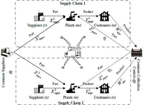
Structure of the CLSC network.
All the transportation processes in the network have been executed via a logistics firm where three different vehicles are used for transportation. All the vehicles have different engines so that their transportation costs, delivery time, and CO2 emissions are different from each other. The capacity of the vehicle is assumed to be limitless. Under these conditions, a few trade-offs should be optimized simultaneously for obtaining a preferred compromise solution.
The developed model can be formulated as a multi-level MILP mathematical model and based on the following assumptions:
- •
Demand is deterministic, and must be fully satisfied.
- •
The capacities of facilities are limited and fixed.
- •
No inventory is allowed in any of the facilities except for the parts in the plants.
- •
There is no disposal after the disassembly.
The developed CLSC model is an extended version of Çalık et al.2. Not all parameters are presented in this paper. Detailed information regarding the previous model can be found at Çalık et al.2
Indices
- i
index of a common suppliers,
- r
index of a suppliers for SC1,
- s
index of a suppliers for SC1,
- m
index of a plants for SC1,
- n
index of a plants for SC2,
- u
index of a customers for SC1,
- v
index of a customers for SC2,
- j
index of a common collection centers,
- c
index of a parts,
- p
index of a vehicle options,
- t
index of a periods.
Parameters
- utcP
unit transportation cost of vehicle p(($/ton) ∙ km),
-
amount of CO2 emission of vehicle p (gr/km),
- CCO2
unit cost of CO2 emission ($/gr),
-
opportunity loss value of part c transported from supplier r to plant m in period t with vehicle p for SC1 (hour),
-
opportunity loss value of part c transported from supplier s to plant n in period t with vehicle p for SC2 (hour),
-
opportunity loss value of part c transported from common supplier i to plant m in period t with vehicle p for SC1 (hour),
-
opportunity loss value of part c transported from common supplier i to plant n in period t with vehicle p for SC2 (hour),
- π
unit opportunity cost of delays when sending parts from suppliers to plants ($/ton ∙ hour),
-
delivery time of part c transported from supplier r to plant m in period t with vehicle p for SC1 (hour),
-
delivery time of part c transported p from supplier s to plant n in period t with vehicle for SC2 (hour),
-
delivery time of part c transported from common supplier i to plant m in period t with vehicle p for SC1 (hour),
-
delivery time of part c transported from common supplier i to plant n in period t with vehicle p for SC2 (hour),
- Nopat
percentage of net profit after tax.
Variables
-
amount of part c transported from supplier r to plant m in period t with vehicle p for SC1 (ton),
-
amount of part c transported from supplier s to plant n in period t with vehicle p for SC2 (ton),
-
amount of part c transported from common supplier i to plant m in period t with vehicle p for SC1 (ton),
-
amount of part c transported from common supplier i to plant n in period t with vehicle p for SC2 (ton),
-
amount of product transported from plant n to customer v in period t with vehicle p for SC2 (ton),
-
amount of product transported from customer u to common collection center j in period t with vehicle p for SC1 (ton),
-
amount of product transported from customer v to common collection center j in period t with vehicle p for SC2 (ton),
-
amount of part c transported from common collection center j to plant m in period t with vehicle p for SC1 (ton),
-
amount of part c transported from common collection center j to plant n in period t with vehicle p for SC2 (ton),
-
if part c transported with vehicle p from supplier r to plant m in period t, 1; otherwise, 0 for SC1,
-
if part c transported with vehicle p from supplier s to plant n in period t, 1; otherwise, 0 for SC2,
-
if part c transported with vehicle p from common supplier i to plant m in period t, 1; otherwise, 0 for SC1,
-
if part c transported with vehicle p from common supplier i to plant n in period t, 1; otherwise, 0 for SC2,
-
if product transported with vehicle p from plant m to customer u in period t, 1; otherwise, 0 for SC1,
-
if product transported with vehicle p from plant n to customer v in period t, 1; otherwise, 0 for SC2,
-
if product transported with vehicle p from customer u to common collection center j in period t, 1; otherwise, 0 for SC1,
-
if product transported with vehicle p from customer v to common collection center j in period t, 1 otherwise, 0 for SC2,
-
if part c transported with vehicle p from common collection center j to plant m in period t, 1 otherwise, 0 for SC1,
-
if part c transported with vehicle p from common collection center j to plant n in period t, 1 otherwise, 0 for SC2,
-
if plant m is open in period t, 1; otherwise, 0 for SC1,
-
if plant n is open in period t, 1; otherwise, 0 for SC2,
- QCjt
if common collection center j is open in period t, 1; otherwise, 0,
-
amount of part c held in plant m in period t for SC1 (ton),
-
amount of part c held in c at plant n in period t for SC2 (ton).
Plants in SC1 → Decision Maker 1 (DM1):
Plants in SC2 → Decision Maker 2 (DM2):
Common Suppliers → Decision Maker 3 (DM3):
Common Collection Centers → Decision Maker 4 (DM4):
Logistics Firm → Decision Maker 5 (DM5):
Constraints
In this model, we handle six different DMs represented as follows: DM1 denotes the Plants in SC1, and the objective function of consists of six components. Components (1)–(6) show the cost of transportation, the cost of CO2 emission, the value of opportunity loss, the cost of purchasing, the fixed opening costs, and the inventory cost of parts, respectively. The objective function of DM2 denoting the Plants in SC2 consists of six components as in DM1. DM3 denotes the Common Suppliers who aim to maximize their profit with the sale of the parts. For the Common Collection Centers, denoted as DM4, the objective function is to maximize the total revenue, which consists of three components. Logistics Firms, denoted as DM5, are responsible for all logistics and transport activities on the network and aim to maximize their profits.
Constraints (18)–(20) are the capacity constraints of suppliers ensuring that the total quantity of parts should be less than the capacity of those suppliers during any period for suppliers at SC1 and SC2, and common suppliers. Constraints (21)–(22) are the production capacity constraints for SC1 and SC2. Constraints (23)–(24) are the demand satisfaction constraints for SC1 and for SC2. Constraint (25) is the constraint capacity of common collection centers. Constraints (26)–(29) are the balance equations for customers SC1 and SC2. Constraints (30)–(31) evaluate the amount of parts held in inventory for SC1 and SC2. Constraints (30)–(34) are the inventory constraints for SC1 and SC2. Constraints (36)–(55) ensure that if there is transportation with a vehicle in line, the corresponding decision variable takes the value of 1; otherwise it takes the value of 0. Constraints (56)–(67) are the non-negativity restrictions, and constraints (68)–(80) are the restrictions on binary variables.
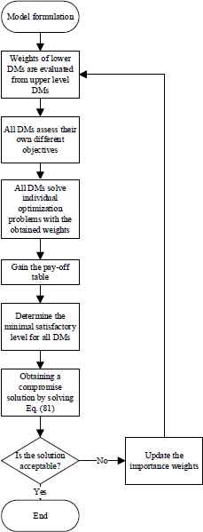
4. The Proposed Novel Interactive Fuzzy Programming Approach
In multi-level programming problems, hierarchy between DMs consists of two levels: the upper-level DMs and the lower-level DMs9, 10. According to the DMs’ behavior, multi-level programming models can be solved by a centralized or decentralized approach. Many decentralized models can perform the solution using Stackelberg game, in which the DM at the first level chooses a strategy followed by the other DMs determining their own strategy. In this game, there is no relationship or cooperation among DMs. Thus, Stackelberg solutions do not satisfy Pareto optimality. To overcome these difficulties, several approaches have been proposed in the literature.
The first approach is developed by Zimmermann15, called the max–min approach. The two-phase fuzzy approach is proposed by Li et al.47. A solution approach based on interactive fuzzy goal programming (IFGP) is proposed by Selim and Ozkarahan34. Another interactive fuzzy approach is proposed by Torabi and Hassini33. Çalık et al.2 also developed a new IFP approach, called the weighted Zimmermann approach based on Fuzzy AHP. After this brief reminder of literature, the steps of the proposed IFP approach can be summarized as follows:
Step 1: Weights of lower DMs are evaluated by using a multi-criteria decision making method such as AHP, ANP, etc. The pairwise comparison matrix can be shown as follows:
where ãij = (lij, mij, uij) is a triangular fuzzy number.The weight vector of the lower-level DMs is obtained by this pairwise comparison matrix. Here, wj shows the relative weight of lower-level DMi. We considered that the importance weight of lower-level DMs could be determined through a decision making process.
Step 2: Individual weights of all DMs’ objectives are obtained by using these weights, and their objectives are optimized as follows:
The upper-level comprises i DMs (DM01, DM02,…, DM0m) [Z0i] and the lower-level comprises j DMs (DM11, DM12,…, DM1n) [Z1j] and l shows the number of objectives. Furthermore,- w0il:
the weight of the objective l of the upper-level DM i,
- w1ul:
the weight of the objective l of the lower-level DM j.
Step 3: According to the weighted sum method, the pay-off table is obtained using the individual objective functions for all DMs.
Step 4: The upper-level DM determines the minimum satisfaction level (δ0) and the lower DMs determine their own minimum satisfaction level based on the upper-level DMs, where the minimum satisfaction level can be denoted as:
Here,- δ0:
the minimum satisfaction level of the upper-level DMs,
-
: the minimum satisfaction level of the lower-level DM j.
Step 5: The following problem is solved and the satisfaction degrees are obtained for all the DMs: maximize
Flowchart of the proposed novel IFP approach.
5. Computational Experiments
In order to assess the performance of the developed CLSC model, a summary of experiments is provided and results are given in this section. Data of the sample problem is based on randomly generated parameters.
5.1. Description of data
With four common suppliers (i = 4), four suppliers in SC1 (r = 3) and SC2 (s = 3), three plants in SC1 (m = 3) and SC2 (n = 3), two customers in SC1 (u = 2) and SC2 (v = 2), two common collection centers (j = 2), three vehicles (p = 3), weight ratios of parts (rc = 0.22, 0.25, 0.15, 0.38) and time periods (t = 3), the developed model is formed. Figure 3 shows the structure of the finished product. The unit CO2 emissions of the vehicles’
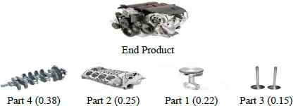
Bill of materials of the finished product.
All of the mathematical formulations are coded in the GAMS-CPLEX 24.0.1 software in a PC equipped with 2.67 GHz processor and 3 GB of RAM. Each of the individual problems of DMs are solved with no more than one CPU second. The solution of the developed model has 4782 variables and 5288 constraints for DM1. When the proposed model is solved with the sample problem, the total cost of DM1 is found to be $5738543.50 for all periods. The results show that the total transportation costs account for a 16% share of the overall cost. While the maximum share is actualized by total purchasing costs with 54%, the minimum share is actualized by total CO2 emissions costs of suppliers, common suppliers, plants, customers and common collection centers with 1%. In the first three periods, 852, 905, and 872 tons of finished products for SC1; 1234, 2086, and 1414 tons of finished products for SC2 are collected with solving DM1’s objective, respectively. Used products are delivered to common collection centers where, after the disassembly process, disassembled parts are transported to the plants. Figure 4 shows the purchased original parts, which are transported from common suppliers and dedicated suppliers to the plants in SC1 and SC2, and used parts that are collected from common collection centers. As seen in Figure 4, while 4484.65 tons of original parts are purchased from common suppliers, plants in SC1 do not purchase any original parts from their own suppliers while minimizing their own objective. The same situation is also true for DM2. In fact, DM2 obtains the minimum total cost by purchasing the original parts from common suppliers. Using the common suppliers, DM1 and DM2 obtain lower objective function values. For the result of maximization of DM3, 27997.86 65 tons of original parts are purchased from common suppliers to each plant. As expected, the maximum amount of purchased original part is obtained by the solution of Z3, while the minimum amount of purchased original part is obtained in the solution of Z2. The logistics firm obtains the maximum profit by carrying 40425.99 tons of material in the network.
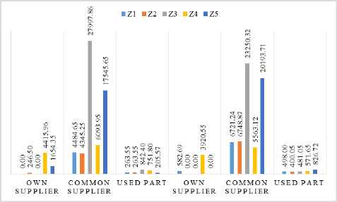
The distribution of parts according to each individual solution.
A preferred compromise solution for DMs is obtained by using three different IFP approaches: SANIIFP’s approach, Çalık et al.’s2 IFP approach, and a novel IFP approach that is presented in this study.
5.2. Solution of the problem with the SANIIFP approach
For getting the membership functions of DMs at both levels for their fuzzy goals for the objective functions, a pay-off table is obtained via solving the individual problems. In this model, five different DMs are handled. Two of them are the upper-level DMs: the plants of common SCs. The others are lower-level DMs: common suppliers, common collection centers, and logistic firm. Initially, individual problems of DMs are solved and the optimal solutions are obtained for all DMs. The pay-off table, which shows the best and worst optimal values for of each individual problem, can be seen in Table 1.
| Z1 | Z2 | Z3 | Z4 | Z5 | |
|---|---|---|---|---|---|
| min Z1 | 5,738,543.50
|
37,897,516.01 | 20,756,053.81 | 1,351,520.17 | 6,974,314.17 |
| min Z2 | 22,978,661.87 | 9,282,576.44
|
13,774,823.07 | 1,749,107.98 | 4,645,485.26 |
| max Z3 | 141,088,964.72 | 122,454,872.57 | 170,314,864.83
|
2,029,625.97 | 37,181,008.35 |
| max Z4 | 41,181,974.71 | 38,365,183.11 | 38,380,952.56 | 3,795,678.44
|
12,767,956.18 |
| max Z5 | 142,816,974.95 | 146,569,980.05 | 135,267,805.01 | 322,043.91 | 81,253,812.11
|
| The worst values | 142,816,974.95
|
146,569,980.05
|
13,774,823.07
|
322,043.91
|
4,645,485.26
|
Pay-off table of each problem.
First, Z1 is minimized using the constraints (1)–(80) for obtaining a lower bound
After solving the main problem (Eq. (87)), the minimal satisfaction level is obtained as 0.47. The satisfaction degrees of the other DMs are obtained as µ1 = µ2 = µ3 = µ5 = α and µ4 = 0.53, respectively.
Here, we assume that the upper-level DMs assess the minimal satisfaction level and update it as
In the second iteration, the minimal satisfaction level is calculated as 0.80 for the upper-level DMs. Then, the lower and the upper bounds of ratio ◿ of satisfaction degree between both levels can be determined as 0.5 and 0.6, respectively. The ratio of satisfaction degrees then becomes
In the third iteration, the ratio of satisfaction degrees is within the specified interval between the two levels calculated as
In the second phase of the approach, the ratios of satisfaction between the upper-level DMs and lower-level DMs are computed in order to obtain a satisfaction balance between the DMs:
Suppose that the upper-level DMs specify different intervals for lower-level DMs. The upper-level DMs determine the interval between the upper-level DMs and DM3, DM4 as [ΔL, ΔU] = [0.6, 0.7], and [ΔL, ΔU] = [0.4, 0.5] for DM5.
While the ratio between DM4 and DM5 is within the interval, the ratio of DM3 is not. Hence, the upper-level DMs specify the satisfaction levels as
The ratios of satisfaction between the upper-level DMs and lower-level DMs are computed as follows:
In the last iteration, the ratio of satisfaction degrees between the DMs is within the specified interval. Furthermore, the upper-level DMs are satisfied in the solution; herewith then the solution becomes the preferred compromise solution and the algorithm stops. At the end of the process, the satisfaction degrees of upper-level DMs are equal to 0.60 and the satisfaction degrees of the lower-level vary between 40% and 70% of the upper-level DMs’ satisfaction degrees.
5.3. Solution of the problem with the IFP approach of Çalık et al.2
The formulation of the Çalık et al.’s 2 approach can be seen as follows:
maximize α0 + w1 · α1 + w2 · α2 + … + wm · αm subject to
In this approach, they consider there are i DMs at the lower-level (DM1, DM2, …, DMm), where A denotes the technology matrix, x indicates vector of the decision variables, and b shows the vector of right-hand side values of the constraints. Moreover, wg indicates the relative importance of the gth objective function, where
the weight of the objective function of the lower-level DM i (i = 1,…, m), the satisfaction degree of the upper-level DM, the satisfaction degree of the lower-level DM i (i = 1,…, m), the satisfaction degree of upper-level DMs’ objective function, the satisfaction degree of the lower-level DM i‘s objective function (i = 1,…, m).
| DM11 | DM12 | DM13 | |
|---|---|---|---|
| DM01 | |||
| DM11 | (1, 1, 1) | (1, 3, 5) | (0.14, 0.2, 0.33) |
| DM12 | (0.2, 0.33, 1) | (1, 1, 1) | (0.2, 0.33, 1) |
| DM13 | (3, 5, 7) | (1, 3, 5) | (1, 1, 1) |
| DM02 | |||
| DM11 | (1, 1, 1) | (3, 5, 7) | (5, 6, 7) |
| DM12 | (0.14, 0.2, 0.33) | (1, 1, 1) | (5, 7, 9) |
| DM13 | (0.14, 0.16, 0.2) | (0.11, 0.14, 0.2) | (1, 1, 1) |
| Aggregation of upper-level DMs judgements | |||
| DM11 | (1, 1, 1) | (1.73, 3.87, 5.91) | (0.84, 1.09, 1.52) |
| DM12 | (0.16, 0.26, 0.58) | (1, 1, 1) | (1, 1.52, 3) |
| DM13 | (0.65, 0.91, 1.18) | (0.33, 0.65, 1) | (1, 1, 1) |
Comparative judgments of the lower-level DMs and aggregated weights.
The triangular fuzzy weights are obtained from Table 2. The outcomes are defuzzified by Center of Gravity (CoG) method and presented as crisp values (0.4901, 0.2574, 0.2524) Using these weights, the following objective function is optimized:
5.4. Solution of the problem with novel IFP approach
Step 1: Taking into account the weights of the lower-level DMs in Section the 5.3, the first step of the novel IFP approach is terminated.
Step 2: All DMs determine their own objectives and the weight vectors are obtained (please see Table 3).
| Decision Makers | Weight vector |
|---|---|
| DM01 | (0.30, 0.5, 0.5, 0.35, 0.10, 0.15) |
| DM02 | (0.30, 0.5, 0.5, 0.35, 0.10, 0.15) |
| DM11 | (1) |
| DM12 | (0.60, 0.30, 0.10) |
| DM13 | (1) |
The weights of all DMs objectives.
According to DM01 and DM02, the most important factors are: the purchasing cost, the transportation cost, the inventory cost, the fixed opening costs, the CO2 emission cost and the cost of opportunity loss, respectively. According to DM12, the purchasing cost, the transportation cost, and the fixed opening costs are the most important factors.
Step 3: We obtain the following pay-off table using the weighted sum method. The membership functions belonging to objectives for DMs are obtained as follows:
Step 4: We assume that DM01 and DM02 specifies the minimal satisfaction level as δ0 = 0.60. Using this value, the satisfaction levels for the lower-level DMs are evaluated:
Step 5: The following problem is solved and the satisfaction degrees are received for all DMs:
By solving Eq. (96), the optimal solutions are obtained. The satisfaction degrees are calculated as: (0.60,0.77) for upper-level DMs, and (0.29,0.60,0.15)for lower-level DMs, respectively. When the proposed IFP approach is compared to SANIIFP, it is obvious that the proposed approach gives an option to the DMs in order to enter their preferences in the solution process.
5.5. Sensitivity analysis
A sensitivity analysis is implemented to see how the satisfaction degrees of the DMs behave when the weight of the lower-level DMs are changed. In other words, we want to investigate the effects of changes in lower-level DMs’ weights, one lower-level DM at a time. In this analysis, according to the specific weight value of one lower-level DM, the weights of other lower-level DMs are obtained proportionally. For instance, the weight of the first lower-level DM (DM11) has been received as 0.4901 When the weight of DM11 is changed from 0.4901 to 0.1, the weights of other lower-level DMs are calculated as follows: The residual sum of weights is 1 − 0.1 = 0.9. This residual value will be distributed to the other DMs proportionally. For DM12, this value is obtained as
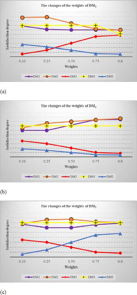
Sensitivity analysis results.
5.6. Comparison of IFP approaches
The developed CLSC model is solved with three different IFP approaches. Comparisons of these approaches are given in Table 5.
| Z01 | Z02 | Z11 | Z12 | Z13 | |
|---|---|---|---|---|---|
| min Z01 | 1,323,494.84 | 12,642,629.38 | 22,461,979.95 | 2,405,531.22 | 7,668,877.08 |
| min Z02 | 7,145,534.54 | 2,166,298.46 | 13,777,240.86 | 1,847,657.89 | 4,635,465.50 |
| max Z11 | 44,849,222.57 | 38,357,400.38 | 170,314,864.83 | 3,976,214.98 | 37,181,008.35 |
| max Z12 | 5,342,885.54 | 16,984,121.55 | 33.121,408.74 | 5,797,374.30 | 15,091,573.76 |
| max Z13 | 44,016,828.30 | 45,285,697.63 | 135,267,805.01 | 5,446,176.25 | 81,253,812.11 |
| The worst values | 44,849,222.57 | 45,285,697.63 | 13,777,240.86 | 1,847,657.89 | 4,635,465.50 |
The pay-off table obtained by the weighted sum method.
| SANIIFP | Ҫalık et al.2 IFP | Novel IFP | ||||||||||
|---|---|---|---|---|---|---|---|---|---|---|---|---|
| Z01 | 60569916.08 | μ01 | 0.60 | Z01 | 57828347.45 | μ01 | 0.62 | Z01 | 18733785.93 | μ01 | 0.60 | |
| Z02 | 64197537.88 | μ02 | 0.60 | Z02 | 57333167.70 | μ02 | 0.65 | Z02 | 12164680.91 | μ02 | 0.77 | |
| Z11 | 79521640.61 | μ11 | 0.42 | Z11 | 88994611.03 | μ11 | 0.48 | Z11 | 59799302.31 | μ11 | 0.29 | |
| Z12 | 1726190.92 | μ12 | 0.40 | Z12 | 3786657.86 | μ12 | 0.55 | Z12 | 4217487.56 | μ12 | 0.60 | |
| Z13 | 23894222.19 | μ13 | 0.25 | Z13 | 7393675.93 | μ13 | 0.04 | Z13 | 16235483.18 | μ13 | 0.15 | |
| Average CPU (s) | 45981901.54 | 0.454 | 43067292 | 0.468 | 22230147.98 | 0.482 | ||||||
| 13.37 | 12 | 32.49 | ||||||||||
Obtained optimal results and satisfaction levels of two IFP approaches.
We observe that the proposed novel IFP approach outperforms the SANIIFP approach and Çalik et al.’s 2 approach for upper-level DMs’. For instance the objective function value of DM01 is obtained as 60569916.08 with SANIIFP, 57828347.45 with Çalık et al. 2, while the optimal solution is obtained as 16096789.54 with the novel IFP approach.
When we compare the satisfaction degrees, we note that the satisfaction degrees for the upper-level DMs raised. The satisfaction degree of DM11 is decreased, while the satisfaction degree of DM12 has increased from 0.4 to 0.6. In different IFP approaches, minimum CPU time is obtained by the novel IFP approach, whereas the maximum CPU time is required by SANIIFP. From Table 5, we see that the proposed novel IFP approach seems to perform better than the SANIIFP and Çalık et al.’s 2 approaches in terms of the values of each objective and satisfaction degrees. In order to reach a preferred compromise solution for all DMs at all levels, we can use IFP approaches for a decentralized multilevel CLSC network problem.
6. Conclusion and Outlook
In this paper, we developed a decentralized multi-level CLSC model with an alliance behavior between two SCs. The developed model consists of two cooperating SCs where common suppliers and common collection centers are allied units for each SC. We focused on the cost of transportation, the cost of CO2 emissions, the cost of opportunity loss, the cost of purchasing, the fixed operating costs and the cost of inventory at the upper-level DMs objectives.
For obtaining a compromise solution for the CLSC model, we applied the SANIIFP approach and a novel IFP approach proposed in this study that is based on Fuzzy AHP. In the first step, upper -level DMs determined the importance of lower-level DMs by using Fuzzy AHP method. Then, in the second step, all DMs at both levels determined the importance of their own objectives. In the third step, we generated the pay-off table by using the weighted sum method. After this step, the upper-level DMs determined the minimum satisfaction level and the lower-level DMs determined their own satisfaction levels using this value. Finally, we solved the model by taking into account Fuzzy AHP weights and minimum satisfaction levels of all DMs.
The main contributions of this article can be summarized as follows:
- (i)
A multi-level mixed integer MILP model with two SCs including common sources, e.g., suppliers and collection centers, and five different DMs is developed. This is the second attempt in literature for investigating the alliance behavior of the CLSC network design.
- (ii)
A novel IFP approach that allows for multiple DMs at the first level and combines their judgments and opinions in an analytically structured method by using Fuzzy AHP has been proposed to solve the CLSC problem. By combining the DMs’ judgments, the minimal satisfaction levels of the lower-level DMs are guaranteed with the value
- (iii)
- (iv)
This paper continues the pioneering work of the authors’ previous article for applying the IFP approach to the CLSC problem with different SCs and common sources.
Acknowledgements
In carrying out this study, the third author, Turan Paksoy, is granted by the Scientific and Technological Research Council of Turkey (TUBITAK) (International Postdoctoral Research Fellowship Program).
References
Cite this article
TY  - JOUR
AU  - Ahmet Çalık
AU  - Nimet Yapıcı Pehlivan
AU  - Turan Paksoy
AU  - Gerhard Wilhelm Weber
PY  - 2018
DA  - 2018/01/31
TI  - A Novel Interactive Fuzzy Programming Approach for Optimization of Allied Closed-Loop Supply Chains
JO  - International Journal of Computational Intelligence Systems
SP  - 672
EP  - 691
VL  - 11
IS  - 1
SN  - 1875-6883
UR  - https://doi.org/10.2991/ijcis.11.1.52
DO  - 10.2991/ijcis.11.1.52
ID  - Çalık2018
ER  -