
Entropy Measures of Probabilistic Linguistic Term Sets
- DOI
- 10.2991/ijcis.11.1.4How to use a DOI?
- Keywords
- Probabilistic linguistic term set; fuzzy entropy; hesitant entropy; total entropy
- Abstract
The probabilistic linguistic term sets (PLTSs) are powerful to deal with the hesitant linguistic situation in which each provided linguistic term has a probability. The PLTSs contain uncertainties caused by the linguistic terms and their probability information. In order to measure such uncertainties, three entropy measures are proposed: the fuzzy entropy, the hesitant entropy, and the total entropy. The fuzzy entropy measures the fuzziness of the PLTSs, and the hesitant entropy measures the hesitation of the PLTSs. To facilitate the computation of all uncertainties contained in the PLTSs, the total entropy is proposed. Some properties and some formulas of the entropy measures are introduced. A multi-criteria decision making model based on the PLTSs is introduced by using the proposed entropy measures. An illustrative example is provided and the comparison analysis with the existing method is given.
- Copyright
- © 2018, the Authors. Published by Atlantis Press.
- Open Access
- This is an open access article under the CC BY-NC license (http://creativecommons.org/licences/by-nc/4.0/).
1. Introduction
Fuzzy sets (FSs)32 have provided great convenience in modeling uncertainties, and have been applied successfully to many fields. Many extensions of FSs were introduced, such as the intuitionistic fuzzy sets1,28, the hesitant fuzzy sets (HFSs)17,18, the dual HFSs36, and the hesitant fuzzy linguistic term sets (HFLTSs)15. The HFSs facilitate decision makers when they are hesitant on providing preferences, which permit multi-valued membership degrees. Under linguistic environment, Rodíguez and Martínez14 provided an overview on the relationship of the process of computing with words and the decision making. Rodíguez et al.13 justified the use of HFLTSs in complex linguistic context. The HFLTSs can similarly permit decision makers to express their qualitative assessments by using several linguistic terms, and they are generally transformed from comparative linguistic expressions close to human’s cognitive process. In order to overcome the limitation of the HFLTSs whose linguistic terms are consecutive, the extended HFLTSs (EHFLTSs)19,22 were introduced, whose linguistic terms may be valued as any term in a linguistic term set. The linguistic terms in the HFLTSs and the EHFLTSs are generally viewed as equally important since no additional information can be obtained from them directly. Liu and Rodíguez9 introduced the fuzzy envelope for HFLTSs to embody the different importance degrees of the linguistic terms in the HFLTSs from an intuitive viewpoint. Zhang et al.33 introduced the possibility distribution assessments based on the expression form of discrete FSs. Such an expression extended the proportional linguistic 2-tuple20 to a more general form, and provided the symbolic proportion of each linguistic term in a linguistic term set, which can be viewed as the original idea of the PLTSs. There are also some research results on the hesitant fuzzy preference relations25,26 and the application of the HFLTSs27.
Recently, Pang et al.12 introduced the probabilistic linguistic term sets (PLTSs) which are composed of the EHFLTSs with each linguistic term having a probability indicating its frequency in group decision making, or the importance of the term, or the degree of belief on that linguistic term expressed by a decision maker. The PLTSs had been investigated from different viewpoints. Bai et al.2 introduced a new comparison method for the PLTSs. Gou and Xu7 proposed some novel operational laws for the linguistic terms, the HFLTSs and the PLTSs. Zhang et al.34 discussed the additive consistency of probabilistic linguistic preference relations based on graph theory. The similar case of the PLTSs in quantitative context was also investigated, and the probabilistic HFSs (PHFSs)30 were introduced, which import probability information to the HFSs. In Ref.30, it was also introduced a consensus building model based on the maximizing score deviation model and aggregation operators for PHFSs. The probabilistic dual HFSs8 were introduced to deal with the risk evaluation problems.
Entropy was originally used to measure the uncertainty contained in a probability distribution. Later on, it was extended to measure the fuzziness contained in a fuzzy set4,10. Pal and Bezdek11 gave a comprehensive review of the entropy of FSs and the methods to combine the fuzziness and probability information of FSs. Under hesitant fuzzy environment, different forms of entropy were proposed. Xu and Xia29 introduced the entropy and cross-entropy for HFSs, and applied the entropy to TOPSIS method in multi-attribute decision making. Farhadinia5 further developed some distance-based entropy measures. Wei et al.21 introduced some new entropy measures which combined both the score function and the deviation function of HFSs into a unified form, and utilized the entropy to compute the criteria weights in multi-criteria decision making. Zhao et al.35 introduced the two tuple entropy which considers both the fuzziness and the nonspecificity of the HFSs.
All of the above entropy measures are suitable for HFSs which have no probability information. New entropy measures should be developed since the probability information in the PLTSs cannot be omitted. Let us consider two PLTSs: L(P)(1) = {s1(0.5), s2(0.5)} and L(P)(2) = {s1(0.01), s2(0.99)} based on a linguistic term set S = {s0,…,s8}. From an intuitive viewpoint it can be seen that they contain different degrees of uncertainty although the linguistic terms used in them are identical. The first PLTS is totally hesitant since both probabilities of the linguistic terms are 0.5, and the second one contains less hesitation since s2 plays an important role because of its high probability and as a result the PLTS behaves like the single linguistic term s2. In this situation, an entropy representing the uncertainties contained in the PLTSs should embody the differences on probability information. In PLTSs, the probability represents the randomness of the appearance of the linguistic terms. Each linguistic term in a PLTS represents a certain degree of fuzziness and multiple linguistic terms in the PLTS represent a certain degree of hesitation if the PLTS contains two or more linguistic terms. To consider all of the uncertainties including probability, fuzziness, and hesitation of a PLTS, and motivated by Refs.21,24,29,35, we propose some new entropy measures which can deal with all of the above uncertainties contained in the PLTSs. We then apply the entropy measures to determine the criteria weights and further develop a multi-criteria decision making model based on the fuzzy TOPSIS method.
The remainder of this paper is organized as follows: Section 2 reviews the PLTSs and entropy measures of HFSs, Section 3 introduces the entropy measures for PLTSs, Section 4 introduces a multicriteria decision making model, Section 5 presents an illustrative example and Section 6 concludes the whole paper.
2. Preliminaries
In this section, some basic concepts including the PLTSs and the entropy measures of HFSs are reviewed.
2.1. PLTSs
The PLTSs are defined by considering probability information in EHFLTSs.
Definition 1. 12
Let S = {s0,s1,…,sg} be a linguistic term set, a PLTS is defined as:
Note that if
In such a way a normalized PLTS is obtained. The set of normalized PLTSs is denoted as
For a PLTS
The distance between two PLTSs was defined based on the distance between each element of the PLTSs, which requires that the number of elements of the two PLTSs to be equal. The method in Ref.12 adds the smallest linguistic term in the shorter PLTS with the probability 0 several times until the shorter PLTS has the same number of elements as the longer PLTS. To avoid the complexity of computation, we propose a new distance between two PLTSs based on the expectation.
Definition 2.
Let L(P)(l), l = 1,2 be two PLTSs, the distance between them is defined as:
2.2. Entropy measures of HFSs
An important issue of the HFS is the measurement of the information contained in it. The commonly-used measure is entropy. Different forms of entropy measures have been proposed for HFSs. Here we mainly review the two tuple entropy which is composed of the fuzziness and nonspecificity of the HFSs.
Definition 3. 35
Let H be the set of HFSs, and EF,ENS : H → [0,1] be two functions, the pair (EF,ENS) is called a two tuple entropy, if it satisfies the following conditions:
- (i)
EF(α) = 0 if and only if α = {0} or α = {1};
- (ii)
EF(α) = 1 if and only if α = {0.5};
- (iii)
EF(α) ⩽ EF(β), if ασ(i) ⩽ βσ(i) ⩽0.5, or ασ(i) ⩾ βσi ⩾ 0.5, # α = # β, i = 1,…,# α;
- (iv)
EF(α) = EF(αc), where αc is the complement of α, which is expressed as αc = ∪αi ∈ α {1 − αi};
- (v)
ENS(α) = 0 if and only if there is only one element contained in α;
- (vi)
ENS(α) = 1 if and only if α = {0,1};
- (vii)
ENS(α) ≤ ENS(β) if |ασ(i) − ασ(j) | ≤ | βσ(i) − βσ(j) | for # α = # β, i = 1,…,# α;
- (viii)
ENS(α) = ENS(αc).
The fuzziness and nonspecificity EF, ENS can be called the fuzzy entropy and hesitant entropy respectively.
3. Entropy measures of the PLTSs
In this section, the fuzzy entropy and hesitant entropy of the PLTSs are introduced, then the total entropy is proposed to combine the two entropy measures.
3.1. The fuzzy entropy of the PLTSs
For any linguistic term li ∈ S, it is easy to transfer the term into a value in [0,1] by using αi = I(li)/g. Since the fuzzy entropy of HFSs can be applied for one value αi ∈ [0,1], we propose the fuzzy entropy of the PLTSs by considering fuzzy entropy of the linguistic terms and the probability information in the PLTSs.
Definition 4.
Let
Let us give some properties of the fuzzy entropy of the PLTSs.
Proposition 1.
The fuzzy entropy defined in the Definition 4 has the following properties:
- (i)
ĒF(s0(1)) = ĒF(sg(1)) = 0, and further ĒF ({s0(p),sg(1 − p)}) = 0;
- (ii)
ĒF(sg/2(1)) = 1;
- (iii)
ĒF(L(P)(1)) ≤ ĒF(L(P)(2)) if
- (iv)
ĒF(L(P)) = ĒF(L(P)c).
Proof.
- (i)
Since α0 = I(s0)/g = 0, αg = I(sg)/g = 1, and EF (0) = EF(1) = 0, thus we have ĒF(s0(1)) = 1 · EF(0) = 0, ĒF(sg(1)) = 1 · EF(1) = 0, and ĒF ({s0(p),sg(1 − p)}) = p·EF(0)+(1 − p)EF(1) = 0;
- (ii)
Since αg/2 = 0.5, EF(0.5) = 1, we obtain that ĒF(sg/2(1)) = 1 · 1 = 1;
- (iii)
If
- (iv)
Since L(P)c = {(sg − li)(pi)|i = 1,…,#L(P)}, and EF(α) = EF(αc), the conclusion ĒF(L(P)) = ĒF(L(P)c) follows naturally.
From the Proposition 1, we can obtain the following property.
Proposition 2.
The proposed fuzzy entropy in Definition 4 coincides with the entropy measure defined in Ref.6 and Ref.23 if pi = 1/(#L(P)).
Proof.
The proof is divided into two parts.
- (i)
It is noted that the linguistic term set used here, S ={s0,…,sg}, is different from the one used in Ref.6, that is, S′ = {s′−τ,…,s′τ}. But they are essentially identical by setting
for li ∈ S, and then we have μ(li) ∈ S′. We need to prove that ĒF(L(P)) in Definition 4 satisfies the conditions of the entropy measure in Ref.6 if pi = 1/(#L(P)). Actually it only needs to prove that 0 ≤ ĒF(L(P)) ≤ 1 sinceand 0 ≤ EF(αi) ≤ 1. The left conditions are the same as in Proposition 1. Thus the result holds. - (ii)
Similarly, we can transform the linguistic term set S = {s0,…,sg} in our proposal to the one used in Ref.23, that is, S″ = {s″0,…,s″g}, by setting ν(li) = li/2, for li ∈ S, and we have í(li) ∈ S″. The proof of the ĒF(L(P)) satisfying the left conditions is straightforward and it is omitted here.
From the above properties, we know that the HFLTSs and the EHFLTSs can be viewed as the special cases of the PLTSs. In a HFLTS HS or an EHFLTS EHS, there are no probability information is provided and thus the linguistic terms can be viewed as equally important. If we impose a probability pi to each term li ∈ HS or EHS, then pi = 1/(#HS) or 1/(#EHS). In this sense, the fuzzy entropy of the PLTSs are more general than the entropy of the HFLTS and the EHFLTSs.
Intuitively, the fuzzy entropy of a LPTS measures the amount of fuzziness contained in it. For an element li(pi) ∈ L(P) = {li(pi)|li ∈ S, i = 1,2,…,#L(P)}, the fuzziness contained in li(pi) is composed of two parts, one is the fuzziness of li, the other is the probability pi. We explain this point by presenting a practical example. Let us consider the safety evaluation of a car based on a linguistic term set S = {s0 : extremely bad,…,sg/2 : medium,…,sg : extremely bad}. If li = s0, pi = 1, then the safety of the car is extremely bad, and the decision may be “not to buy”. If li = sg, pi = 1, then the decision may be “buy” since the safety of the car is extremely good. If li = sg/2, pi = 1, then the decision may be hesitant between “buy” and “not to buy” since the safety lies in the margin of good and bad. This case shows that the linguistic term li may bring some fuzziness. On the other hand, if pi = 0, then li will not appear, and if pi = 1, then li will appear and the fuzziness of li(pi) is solely determined by li. If 0 < pi < 1, then li may appear or not, and since li contains fuzziness itself, the fuzziness of li(pi) is determined by pi and li collectively. By summarizing the fuzziness of all elements in L(P), we can obtain the fuzziness, i.e., the fuzzy entropy of L(P).
For an element li0(pi0) ∈ L(P), if pi0 → 1, then pj → 0, j ≠ i0 and ĒF(L(P)) → EF(αi0), which indicates that li0(pi0) plays an important role in de termining the fuzzy entropy of L(P). Similarly, if pi0 → 0, then pi0 · EF(αi0) → 0, which means that the importance of li0(pi0) is almost negligible in L(P). These results are consistent with the intuition that the linguistic terms with low probability are less important than the terms with high probability in a PLTS.
The expression of ĒF depends on the form of EF. In Ref.11, it was given some formulas of entropy, based on which, we propose the following fuzzy entropy measures of PLTSs:
The properties of EF were deeply investigated and for more details we refer to Ref.11.
It is interesting that a new entropy can be constructed as a function of some known entropy measures6. Motivated by this idea, we can construct a new fuzzy entropy in the following form:
Based on this idea, a special fuzzy entropy can be obtained as a convex combination of the aforementioned six fuzzy entropy measures, that is,
To illustrate the computational process of the fuzzy entropy, we provide an example as follows:
Example 1.
Let S = {s0,s1,…,s8} be a linguistic term set, and
be three normalized PLTSs. For simplicity, we set the parameters in the fuzzy entropy measures as: q = 1 in
| L(P)(1) | L(P)(2) | L(P)(3) | |
|---|---|---|---|
|
|
0.9818 | 0.9056 | 0.9300 |
|
|
0.9000 | 0.7500 | 0.7500 |
|
|
0.9761 | 0.8794 | 0.9098 |
|
|
0.9000 | 0.7500 | 0.7500 |
|
|
0.9980 | 0.9500 | 0.9634 |
| 0.9873 | 0.9330 | 0.9506 | |
| ĒF | 0.9600 | 0.8613 | 0.8757 |
The computation results of the fuzzy entropy.
From the results, we can see that except for
for l = 1, 3, 5, 6.
The arithmetic mean of all the entropy measures also produce the same ranking. If q = 1 in
Thus they cannot discriminate L(P)(2) and L(P)(3).
Let us investigate
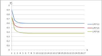
The functions of
If q > 1 in
The result is not the same as most of the other entropy measures. This can be proved in a brief way.
Actually, if a > b > 0, we have
Therefore, if q → +∞, then
It can be obtained that β(1) = 0.6, β(2) = 0.5, β(3) = 0.375, and β(1) > β(2) > β(3), and thus
All of the above results can be seen from Fig. 1.
From the example, we can see that sometimes the computational results of the fuzzy entropy measures are not consistent. To avoid this drawback we recommend the use of the convex combination of such fuzzy entropy measures.
In the more general cases, Pal and Bezdek11 defined the multiplicative and additive classes of entropy measures. Here we review them briefly.
Let f : [0, 1] → R+ be a function satisfying f′(x) > 0, f″(x) < 0, and
Based on these results, we can obtain a new class of fuzzy entropy of the PLTSs. Let
3.2. The hesitant entropy of the PLTSs
The hesitant entropy defined in Definition 3 cannot consider the probability information in the PLTSs. Therefore, in the following we redefine the hesitant entropy for PLTSs which can deal with the probability and the hesitation contained in the PLTSs.
Definition 5.
Let
- (i)
ĒH(L(P)) = 0 if and only if L(P) = {l1(1)}, that is, L(P) only contains one element;
- (ii)
If L(P) = {l1(p1), l2(p2)}, and p1 → 1, p2 → 0, then ĒH(L(P)) → 0;
- (iii)
ĒH(L(P)) = 1 if and only if L(P) = {s0(0.5), sg(0.5)};
- (iv)
ĒH(L(P)(1)) ≤ ĒH (L(P)(2)), if #L(P)(1) = #L(P)(2), P(1) = P(2), and
- (v)
If L(P) = {l1(p1), l2(p2)}, and γ12 → 0, then ĒH(L(P)) → 0;
- (vi)
ĒH(L(P)) = ĒH(L(P)c).
By considering the above conditions, we can give the hesitant entropy of the PLTSs as:
The hesitant entropy measures the deviation of the linguistic terms in the LPTS and also considers the probability information of such terms. For li(pi), lj(pj) ∈ L(P), i ≠ j, the bigger the deviation of li and lj, i.e., the value of γij, the bigger the hesitancy contained in L(P). On the other hand, the biggest hesitancy achieves when pi = pj, since in this case li,lj have the same probability to appearance. Adding the hesitancy of any pairs in L(P) we can obtain the overall hesitancy, i.e., the hesitant entropy of L(P).
In the following we prove that the ĒH(L(P)) expressed by the Eq. (14) meets the requirements in Def. 5.
Proposition 3.
The ĒH(L(P)) expressed by the Eq. (14) is a hesitant entropy.
Proof.
It only needs to prove that the ĒH(L(P)) satisfies the following conditions:
- (i)
If L(P) = {l1(1)}, then it is obvious that ĒH(L(P)) = 0.
By using reduction to absurdity, we assume that there exist at least two different elements l1(p1),l2(p2) ∈ L(P), and ĒH(L(P)) = 0. In this case, ĒH(L(P)) ≥ 4p1p2 f (γ12). Therefore, we can obtain that p1 = 0 or p2 = 0, or f (γ12) = 0. As a result, one element does not exist or the two elements are identical, which contradicts the assumption. Thus ĒH(L(P)) = 0 leads to the conclusion that L(P) = {l1(1)}. ĒH(L(P)) = 0 if and only if L(P) = {l1(1)}, that is, L(P) only contains one element;
- (ii)
If L(P) = {l1(p1), l2(p2)}, and p1 → 1, p2 → 0, then ĒH(L(P)) = 4p1p2 f (γ12) → 0;
- (iii)
If L(P) = {s0(0.5),sg(0.5)}, then ĒH(L(P)) = 4 · 0.5 · 0.5 · 1 = 1. If ĒH(L(P)) = 4p1p2 f (γ12) = 1, then we have 4p1p2 f (γ12) ≤ 4p1p2 ≤ 4(p1 + p2)2/2 ≤ 1, and the equation holds when p1 = p2 = 0.5, and we have f (γ12) = 1 which leads to the conclusion that γ12 = 1. Therefore L(P) = {s0(0.5),sg(0.5)};
- (iv)
The conclusion follows naturally because of the monotonicity of the function f and the assumption that P(1) = P(2);
- (v)
If L(P) = {l1(p1), l2(p2)}, and γ12 → 0, then ĒH(L(P)) = 4p1p2 f (γ12) → 0;
- (vi)
We assume that
Proposition 4.
The proposed hesitant entropy in Definition 5 coincides with the hesitant entropy defined in Ref.23 if pi = 1/(#L(P)).
Proof.
If pi = 1/(#L(P)), then
From Definition 5 we know that ĒH(L(P)) satisfies the conditions of the fuzzy entropy in Ref.23.
The regular increasing monotone (RIM) function31 used in the calculation of OWA weights satisfies the requirements of hesitant entropy. There are actually numerous such functions can be found in the literature. In the following we only give several simple examples:
The hesitant entropy measures of PLTSs generated from fl(x) are denoted as
In the similar way as the fuzzy entropy, a new class of hesitant entropy can be constructed by using the convex combination of the above examples, that is,
To demonstrate the behavior of the hesitant entropy, we present a numerical example.
Example 2.
Let L(P)(l), l = 1,2,3 be the same as in Example 1. Set r = 1 in
| L(P)(1) | L(P)(2) | L(P)(3) | |
|---|---|---|---|
|
|
0.1200 | 0.2500 | 0.1875 |
|
|
0.1873 | 0.3827 | 0.2908 |
|
|
0.0184 | 0.0761 | 0.0382 |
|
|
0.1631 | 0.3219 | 0.2504 |
|
|
0.0869 | 0.1892 | 0.1378 |
|
|
0.2133 | 0.4000 | 0.3222 |
| ĒH | 0.1305 | 0.2700 | 0.2045 |
The computation results of the fuzzy entropy.
From the results, we can see that all the hesitant entropy measures produce the same ranking as
Additionally, the hesitant entropy of L(P)(2) is greater than L(P)(1) since it has more hesitation both in linguistic terms and the probability. The hesitant entropy of L(P)(2) is greater than L(P)(3) since it is totally hesitant on s2 and s4, while L(P)(3) is not so hesitant since s3 plays a major role because of its high probability and s2 and s4 influence the hesitation to a less content. The reason that the hesitant entropy of L(P)(3) is greater than L(P)(1) seems to be very obvious since it contains more hesitation both on the linguistic terms and the probability. These observations fit well with our intuition.
3.3. The total entropy of PLTSs
The fuzzy entropy and hesitant entropy measure the fuzziness and hesitation contained in PLTSs respectively. They reflect different uncertain information of the PLTSs but they determine the total uncertainties contained in the PLTSs collectively. In this section, we develop a total entropy of PLTSs which combines the fuzzy entropy and the hesitant entropy in a unified form. Compared with the two tuple entropy35, such a form will facilitate the computation of the entropy.
Definition 6.
Let
- (i)
ĒT (L(P)) = 0 if and only if L(P) = {s0(1)} or L(P) = {sg(1)};
- (ii)
ĒT (L(P)) = 1 if and only if L(P) = {sg/2(1)} or L(P) = {s0(0.5),sg(0.5)};
- (iii)
ĒTL(P)(1) ≤ ĒT (L(P)(2)), if ĒF (L(P)(1)) ≤ ĒF(L(P)(2)), and ĒH(L(P)(1)) ≤ ĒH(L(P)(2));
- (iv)
ĒT (L(P)) = ĒT (L(P)c).
Proposition 5.
The proposed total entropy in Definition 5 coincides with the total entropy defined in Ref.23 if pi = 1/(#L(P)).
Proof.
If pi = 1/(#L(P)), then the PLTS L(P) can be viewed as an EHFLTS in which the linguistic terms are retained and the probabilities are deleted. We prove the ĒH(L(P)) satisfies the conditions of the total entropy in Ref.23.
- (i)
It is obvious that ĒT (L(P)) = 0 if and only if L(P) = {s0(1)} or L(P) = {sg(1)};
- (ii)
If L(P) = {sg/2(1)}, then ĒT (L(P)) = 0;
- (iii)
Suppose that
- (iv)
It is obvious that ĒT (L(P)) = ĒT (L(P)c).
This completes the proof.
From the above property, we know that the total entropy introduced here is more general than the one in Ref.23 since the probability of each linguistic term may not be equal. Additionally, the total entropy introduced here has more desirable properties than the one in Ref.23 regarding the probability information.
By considering the conditions in Definition 6, and the properties of the fuzzy entropy and the hesitant entropy, we can construct the total entropy as ĒT (L(P)) = ψ(ĒF(L(P)), ĒH(L(P)), where ψ: [0,1] × [0,1] → [0,1]. Note that the fuzzy entropy and the hesitant entropy can be viewed as two parallel concepts for PLTSs, thus they are commutative in the definition of the total entropy. Considering this notice and the properties of the fuzzy entropy and the hesitant entropy, the conditions in Definition 6 reduce to the following properties of the function ψ:
- (i)
ψ(0,0) = 0;
- (ii)
ψ(1,0) = ψ(0,1) = 1;
- (iii)
ψ(x,y) = ψ(y,x);
- (iv)
ψ(x,y) is monotone increasing with respect to x and y.
Since the fuzzy entropy and the hesitant entropy of PLTSs are invariant with respect to a PLTS and its complement, the last requirement of the total entropy means that ψ(x,y) = ψ(x,y), which is trivial. Additionally, if one of the fuzzy entropy and the hesitant entropy approaches 0, then the total entropy will approach the other entropy. That is to say, ψ(x,y) → x if y → 0, and ψ(x,y) → y if x → 0.
Let us consider a special case that ĒF(L(P)) → 1, ĒH(L(P)) → 1. For the simple case that L(P) = {l1(p1),l2(p2)}, we have
Since p1 + p2 = 1, then we know that EF (α1), EF(α2) → 1, and thus l1,l2 → sg/2. On the other hand, since ĒH(L(P)) = 4p1p2 f (γ12) → 1, we have p1, p2 → 0.5, and f(γ12) → 1, thus l1 → s0, l2 → sg, which contradicts with l1, l2 → sg/2. Therefore, the value ψ(1,1) has no practical meaning and it can be left undefined. To be convenient for the denotation of the function ψ, ψ(1,1) can also be set as any value in [0,1], for example as the value 1. The assumption will not influence the rationality of the function.
It is interesting that the triangular co-norm3 satisfies all the conditions of the total entropy. For simplicity, we only give the following commonly-used triangular co-norms:
By replacing x with ĒF(L(P)), and y with ĒH(L(P)), we can obtain the expression of the total entropy. The corresponding total entropy generated from the function ψl(x,y) is denoted as
4. Multi-criteria decision making model based on PLTSs
In this paper, we consider the linguistic multicriteria decision making problem that consists of a finite set of alternatives A = {a1,…,am}, and a set of criteria C = {c1,…,cn} with the weighting vector W = (w1,…,wn) being completely unknown. A group of decision makers provide their assessments of each alternative with respect to the criteria, and each element of the collective assessment matrix is composed of several linguistic terms, each of which has a probability that is generated by the frequency of that term in the group opinions. After normalization, an assessment matrix based on PLTSs is obtained as
In the following, we introduce the resolution process based on the fuzzy TOPSIS method16.
Step 1. Compute the average total entropy under each criterion cl, l = 1,…,n as:
Step 2. Compute the weights of the criteria as
The idea of the above method lies in the fact that the less uncertainties contained in the assessments under the criterion, the more important of the criterion, and thus the bigger weight it should have.
Step 3. Calculate the fuzzy positive ideal solution
Step 4. Compute the closeness coefficient (CC) of each alternative as
Step 5. Rank the alternatives according to their CCs and select the biggest one as the solution.
Remark 1.
By simple computation in Step 3, we have d+(ak) + d−(ak) = 1. Actually,
Therefore, in Step 4 we have CCk = d− (ak), and Step 4 can be omitted.
5. An illustrative example
For convenience of comparison, in this section we adopt the illustrative example in Ref.12. The directors of a company want to invest on three projects A = {a1,a2,a3}, and each project is evaluated from four criteria C = {c1,c2,c3,c4} based on a linguistic term set {s0,s1,…,s8} by using the Balanced Scorecard method with the criteria weights being completely unknown. After collecting the assessments of the directors and a normalization process is further conducted, the following assessment matrix based on PLTSs is obtained as in Table 3.
| c1 | c2 | c3 | c4 | |
|---|---|---|---|---|
| a1 | {s3(0.4),s4(0.6)} | {s2(0.2),s4(0.8)} | {s3(0.2),s4(0.8)} | {s3(0.4),s5(0.6)} |
| a2 | {s3(0.8),s5(0.2)} | {s2(0.25),s3(0.5),s4(0.25)} | {s1(0.25),s2(0.5),s3(0.25)} | {s3(0.8),s4(0.2)} |
| a3 | {s3(0.6),s4(0.4)} | {s3(0.75),s4(0.25)} | {s3(0.33),s4(0.33),s5(0.33)} | {s4(0.8),s6(0.2)} |
The normalized assessment matrix12.
The problem is solved by the following steps in the previous section.
Step 1. Compute the average total entropy of each criterion. There are six formulas of the fuzzy entropy, six formulas of the hesitant entropy, and four formulas of the total entropy introduced in this paper. Therefore, we have 6 × 6 × 4 = 144 different combinations of the total entropy. Since some entropy measures contain parameters, there are actually infinite formulas of total entropy, and we cannot explore all of the cases. For simplicity, we adopt the arithmetic mean of the fuzzy entropy, the hesitant entropy and the total entropy expressed by Eqs. (10), (21) and (26) respectively.
Assume that the parameters in the entropy measures are given as q = 1 in
| ĒF | ĒH | ĒT | W | |
|---|---|---|---|---|
| c1 | 0.9294 | 0.1453 | 0.9673 | 0.1736 |
| c2 | 0.9006 | 0.1600 | 0.9543 | 0.2425 |
| c3 | 0.8355 | 0.1780 | 0.9242 | 0.4022 |
| c4 | 0.9249 | 0.1757 | 0.9657 | 0.1817 |
The computation results of the entropy measures and the criteria weights.
Step 2. Compute the weighting vector W of the criteria and the result is shown in Table 4.
Step 3. Calculate the distance between each alternative and the fuzzy positive ideal solution or fuzzy negative ideal solution as (d−(a1), d−(a2), d−(a3)) = (0.4737, 0.3379,0.4733).
Step 4. Rank the alternatives according to their CCs as a1 ≻ a3 ≻ a2, and the best choice is a1.
It can be seen that our result produces the same ranking as the extended TOPSIS method and the aggregation method in Ref.12. In fuzzy TOPSIS method, the ranking of alternatives is determined solely by the weights of criteria when the assessments of each alternative under the criteria are fixed. Although the criteria weights of our method and Ref.12 are different, they have a common characteristic that the ranking of the criteria weights is the same, i.e., w3 > w2 > w4 > w1. Therefore, the reason for the same ranking of alternatives lies in the same ranking of criteria weights. The Ref.12 utilized the optimization model by maximizing the deviation of the weighted assessments of alternatives under each criterion to compute the criteria weights. Our method seems to be more direct and flexible, which computes the criteria weights by using the entropy measure of the assessments under each criterion. Such entropy measures deal with PLTSs in a comprehensive way by considering the probability, the fuzziness and the hesitation contained in the PLTSs, and different forms of entropy can be selected by different decision makers.
6. Conclusions
In the situation that includes both hesitation and probability information, the PLTSs serve as a good tool to consider both information. The PLTSs contain probability, fuzziness and hesitation information, which can be measured by fuzzy entropy and hesitant entropy respectively, and both entropy measures can be combined into the total entropy. This paper discusses different forms of such entropy measures and applies them in the multi-criteria decision making. In the future, more forms of the entropy measures will be further investigated, and new applications of the entropy will be studied.
Acknowledgments
The authors are very grateful to the Editor and the anonymous reviewers for their constructive comments and suggestions that have helped to improve the quality of this paper. This work is supported by the National Natural Science Foundation of China (71571123); the Key Scientific Research Funds of Henan Provincial Department of Education (15A630011, 16A630038, 17A120006); the Doctoral Research Start-up Funding Project of Zhengzhou University of Light Industry and Henan University of Economics and Law (BSJJ2013053, 800234); the Pre-Research Funds on National Key Projects of Henan University of Economics and Law (852014).
References
Cite this article
TY  - JOUR
AU  - Hongbin Liu
AU  - Le Jiang
AU  - Zeshui Xu
PY  - 2018
DA  - 2018/01/01
TI  - Entropy Measures of Probabilistic Linguistic Term Sets
JO  - International Journal of Computational Intelligence Systems
SP  - 45
EP  - 57
VL  - 11
IS  - 1
SN  - 1875-6883
UR  - https://doi.org/10.2991/ijcis.11.1.4
DO  - 10.2991/ijcis.11.1.4
ID  - Liu2018
ER  -