
Facial Peculiarity Retrieval via Deep Neural Networks Fusion
- DOI
- 10.2991/ijcis.11.1.5How to use a DOI?
- Keywords
- face retrieval; clustering analysis; ASM; deep learning; DNN
- Abstract
Face retrieval is becoming increasingly useful and important for security maintenance operations. In actual applications, face retrieval is usually influenced by some changeable site conditions, such as various postures, expressions, camera angles, illuminations, and so on. In this paper, facial peculiar features are extracted and classified by dynamically integrated deep neural networks (DNNs), in order to enhance the adaptability in actual conditions. Firstly, eight kinds of facial components are detected and located by clustering analysis and Active Shape Model (ASM). Secondly, certain peculiar patterns are defined for each kind of facial component, and eight specialized DNNs are designed to extract features and classify components. Thirdly, the similarity between faces is calculated by dynamically integrating the results of each DNN. Comparative experiments on standard image sets and wild image sets demonstrate that our algorithm outperforms global feature models in retrieval accuracy. Our algorithm is particularly suitable for practical application with regard to natural real videos and images.
- Copyright
- © 2018, the Authors. Published by Atlantis Press.
- Open Access
- This is an open access article under the CC BY-NC license (http://creativecommons.org/licences/by-nc/4.0/).
1. Introduction
Video monitoring systems have been employed in the field of security worldwide, and face retrieval has become one of the well-studied problems in computer vision. Finding coincident faces from captured videos or images remains a challenge and requires development. Although videos can provide more information than a single image1, and several existing methods have performed impressively on face retrieval2,3, these methods are primarily developed and tested by using either strictly controlled footage or high-quality video images. Faces in these materials are often collaborative and shot under simple lighting and viewing conditions, and videos or images are screened and stored in high-quality format.
Videos in practical repositories are different, because they are used to record real scenes such as streets, public squares, bus or train stations, airports, etc. Such videos are typically characterized by changeful postures and complex lighting conditions, and are often corrupted by motion blur. Bandwidth and storage limitations may result in compression artifacts that make face retrieval even more difficult.
Some effective face recognition algorithms have been studied by many groups such as Google, Face++, etc. We pay attention apart from others to face retrieval from actual constrained monitoring videos or images, and we propose a novel framework at the base of facial peculiarity and deep learning, as shown in Fig. 1.
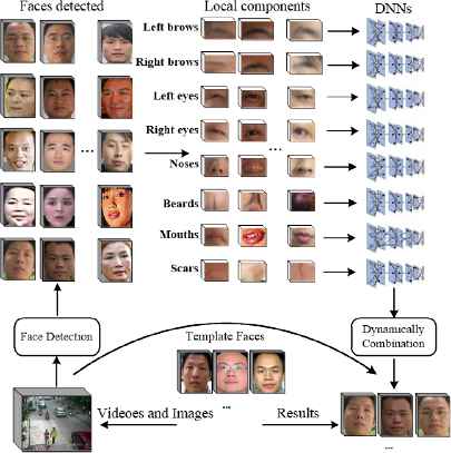
Framework of our algorithm. Eight kinds of components are chosen for the operation: left brow, right brow, left eye, right eye, nose, mouth, beard, and visible scars or birthmarks. The first six are detected and located by ASM from videos or images, and the last two are obtained by checking correlative areas of faces. For videos of known categories, the obtained components are classified accordingly and used to train DNN models. The template face and unknown faces are handled separately, and the results are dynamically integrated to calculate the complete similarity for the retrieval.
The contributions of this study are summarized as follows:
- (1)
Clustering analysis is implemented to reduce the target region, so that the face detection and facial component location can be accelerated.
- (2)
The peculiar features of components are distinct and stronger than those of entire faces.
- (3)
A robust model by DNN is used to classify facial components. This model is more effective in extracting high-level features than traditional neural networks with fewer layers.
- (4)
A dynamic method is introduced to synthesize multiple DNNs. This method can effectively reflect the peculiar intensities of different components.
2. Related work
Previous research focused on searching face targets obtained from different modalities. For example, an original face image is converted into a corresponding sketch image, after which recognition is conducted by sketches4,5. Such a method can simplify the facial features, but the sketch extraction may be influenced easily by illumination. Certain handcrafted descriptors, such as local binary pattern (LBP), scale invariant feature transform (SIFT), and histogram of oriented gradients (HOG)6,7,8 have the effect of comparing faces, but they generally consider the features of the whole face and are easily disturbed by postures and illuminations. Boosting methods are used to detect facial key points9,10, because such methods can accurately locate the face. However, many such studies are used as bases of controlled image sets in laboratories, such as MultiPIE and FERET benchmarks11,12, in which the image-forming condition is strictly controlled. The condition is considerably more complex in fact.
For faces with posture and lighting variation, 3D models are used to revise an off-axis image to a frontal image and to standardize lighting suitable for comparison13,14, and 15. Although these methods may have reliable effects, they are time consuming and typically require additional and special imaging equipment.
Deep learning, a class of machine learning techniques mainly developed since 2006, has been applied for face classification. Deep learning generates numerous stages of nonlinear information processing in hierarchical architectures, which are employed in feature learning and pattern classification16. Typical models contain deep belief network, restricted Boltzmann machine, deep Boltzmann machine, DNN, and related unsupervised learning algorithms such as auto encoders17 and sparse coding18. These methods are used for higher-level feature representations and classification19,20. In recent years, some famous companies and research teams have used DNN for face detection or recognition, such as Facebook’s DeepFace21, Yahoo’s Deep Dense Face Detector22, Google’s FaceNet23, and so on. Generally, deep learning methods turn a global face image as input data, and face analysis is accomplished internally. On the one hand, this process shows the intelligent advantage of deep learning, on the other hand, feature extraction of a whole face increases the complexity of networks. Retrieval accuracy may be influenced, particularly when the videos and images are obtained from actual applications.
In this study, we propose a robust and useful algorithm, which takes advantage of deep learning with peculiarities of facial components.
3. Facial component location
For facial component location, Active Shape Model (ASM) is a classic algorithm introduced by Cootes24 and improved by other researchers over the past few years. ASM is used to automatically locate landmark points that define the shape of any statistically modeled object from an image. When modeling faces, the landmark points lie along the shape boundaries of facial components such as eyebrows, eyes, nose, lips, and so on. Searching the best candidate feature points by traditional ASM needs long time. In this paper we propose improvement approaches to increase the rate.
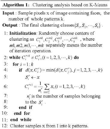
To strengthen the adaptability of global variations, some pre-treatments are needed, such as adjustment and normalization of global brightness. And then considering face usually has conformable local gray value, while other regions have diverse gray value, such as textures and graphic patterns on clothes, we should take advantage of the gray-similarity to detect possible areas. Clustering analysis can achieve the pattern recognition based on the similarities to judge automatically25, so we actualize the clustering analysis by K-Means, in order to reduce the object regions of ASM. The process is expounded as follows:
By these treatments, the searching range of ASM can be reduced, and the whole process can achieve higher speed. The location of facial component is annotated on training image set. Supposing that there are n face images in the training set and each face has m landmark points, the shapes can be represented by vectors
Here
By aligning faces in set X , we can get the new set
And the average template of face is
The deviation between samples and average template can be calculated as
And the covariance matrix is
We assume the nonzero eigenvalue vector and eigenvector are λi and pi, then a face shape can be represented as
Here Pt = (p1,p2,…,pt) is a matrix of the first t eigenvectors of the covariance matrix, and Bt = (b1,b2,…,bt) is a vector that indicates the variation from X to
By steps above, face shapes in videos and images can be searched and extracted, and then facial components can be located with the help of landmark points. Several examples are presented in Fig. 2.
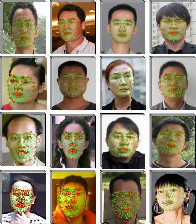
Examples of facial component location. Red points mean the landmark points of facial components. After facial component location, it is necessary to increase the consistency of images. This task is conducted by aligning, which includes translocation, zooming, and rotation.
4. Face retrieval by dynamically integrated DNN
DNN is a deep learning model that functions as both feature extractor and classifier. For feature extraction, it maps specific pixels from an input image into a general and hierarchical feature vector. The feature vector can be classified by several fully connected layers26,27. In contrast to traditional methods, DNN has higher artificial intelligence, that is, certain functions and parameters can be optimized inside automatically but not artificially by training, and better effects and higher efficiency can be achieved. In this paper, features of separate facial component are extracted by traditional DNN at first, and then, an innovative fusion structure is proposed to dynamically integrate the results of each DNN.
Generally, DNN has a succession of layers, including an input layer, an output layer, and several hidden layers with multiple units. The input layer is the image data, the output layer is the result, and each hidden layer generates mapping vectors. Every layer directly links only to the one behind it except the output layer. The data in each layer is transformed by convolutional function, which is related to the activeness of the corresponding units in its layer. According to the training process, the adjustable parameters of DNN are jointly optimized by minimizing misclassification error. The structure of DNN is shown in Fig. 3.
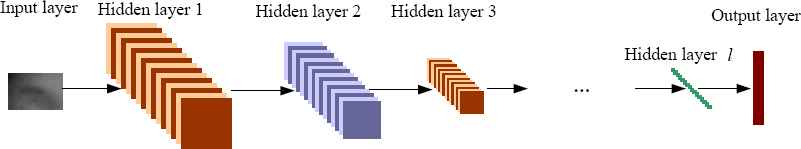
The structure of single DNN
We suppose that the unit j in layer n is
Here n is the layer index; Y is a map of size Mw × Mh, Wij is the weight vector between layer n and layer n + 1,
In layer n − 1, the output map Yn−1 with the size of
In the last layer l + 1, the final output is:
The activation function f depends on the supervised task that the network must achieve. Typically, it is the identity function for a regression problem and is named softmax function, as follows:
In this formula, L represents the whole number of patterns to be classified.
By training on a known image set, the final output layer is down sampled to one pixel or a one-dimensional feature vector. The training process can be conducted as follows:
For face retrieval, the images of eight kinds of facial components are sent to corresponding DNNs and later provide eight classification results of the components. The similarity between the detected face and template face can be calculated upon synthesis of single results. Therefore, a key concern is how to optimize the combination of outputs from various DNNs. The common operation is simply averaging the outputs. In our algorithm, all DNNs with dynamic weights are integrated, and we take the different significance of every facial component into account. The process is presented in Fig. 4.
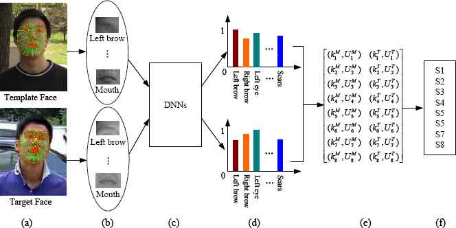
The whole procedure of face retrieval by dynamically integrating several DNNs. (a) The original images including faces. (b) Facial components detected and located from template and target faces. (c) Feature extraction and classification for each kind of component by corresponding DNN. (d) Classification of different kinds of peculiar components, here the color of column means different kind of components, and the height of column means the weight value of current classification. (e) Vectors of classification results with dynamic weights generated from template and target faces. (f) Calculating the whole similarity for face retrieval.
For component Ci, the DNN is Ni, and the component is classified to pattern p, with the weight Ui. For pattern p, the final standard mapping vector is
The whole difference of the face is:
K is the whole pattern kind valued as 8 in this study. In this paper, every facial component can extract a local likelihood, and then they are fuzzily polymerized with dynamic weights, so we call the factor as “fuzzy weight factor”, which is m, typically has a value ranging from 0 to 5.
If the face is similar to the template, the Jm becomes smaller, so the given expression must meet the following conditions:
Based on Lagrange steepest descent method, the best weight can be calculated as:
Based on the preceding operation, the detected face components and template facial components are separately sent into the DNNs before their classification results and weights can be obtained. Thus, the similarity vector is formed as:
5. Experimental results and analysis
We have tested the new algorithm on a personal computer that has an Intel Core CPU with 3.33 GHz and 8GB DDR.
For full contrast, our experiments are operated on two types of image sets: standard dataset in which the illumination, expression, and angle are strictly controlled; and natural dataset in which the images are captured from wild videos.
5.1 Datasets of standard faces
We test our algorithm on a number of public standard datasets, including
- (1)
ORL28, which contains 400 images of 40 subjects taken with varying poses and expressions;
- (2)
Extended Yale B database29, which mainly tests illumination robustness of face recognition algorithms, containing 38 subjects, with 64 frontal images per subject taken with strong directional illuminations;
- (3)
CMU PIE30, which has the same random partition described in our experiments; and
- (4)
Multi-PIE database11, which consists of images of 337 subjects at a number of controlled poses, illuminations, and expressions taken over four sessions. Each standard face image set is partitioned through random selection of half the set per subject for training and the rest for testing. For contrast, several popular algorithms are chosen, such as MKL31, learning-based descriptor32, simile classifier33, background sample34, associate-predict model35, mid-level feature36, visual attributes37, and classic DNN for entire face, which is one of the hot research directions currently. All of these algorithms are used to work on the same set of data. Table 1 presents the results.
The contrast shows the accuracy of our method is top-ranked on standard datasets.
| Method | Accuracy(%) |
|---|---|
| MKL | 85.2 |
| Learning-based Descriptor (LD) | 92.3 |
| Simile Classifier (SC) | 88.7 |
| Background Sample (BS) | 90.1 |
| Associate-predict Model (AM) | 86.6 |
| Mid-level Feature (MF) | 88.3 |
| Visual Attributes (VA) | 89.5 |
| DNN for Entire Face (DNN-EF) | 91.3 |
| ours (DNNs-Fusion) | 91.6 |
Retrieval accuracy on standard datasets.
5.2 Dataset of unconstrained faces
We further test our algorithm on the more challenging faces in the Pubfig image set. Pubfig, built by Columbia University, contains 58,797 images of 200 persons; all of the images are captured from natural videos and pictures37.
Similarly, half of the Pubfig images are used for training and the rest are used for testing. We also choose the same algorithms for contrast. The performances are shown in Fig. 5.
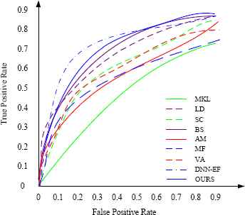
True positive rate and false positive rate test on the wild image set of Pubfig
In this experiment, our algorithm can achieve higher true positive rate and its false positive rate is lower than that of other algorithms.
5.3 Computational cost
From a computational cost perspective, we see that the overall calculation is related to the number of layers in DNNs because of the convolution operations in the hidden layers. In this paper, our DCDNN consists of eight parallelizable DNNs, each of which has seven layers. Based on the hardware and test on Pubfig mentioned in section 5.2, the mean CPU time used by our algorithm is approximately 0.12 second per image. For comparison purposes, the other algorithms use up the following time: MKL, 0.1 second per image; learning-based descriptor, 0.15 second per image; simile classifier, 0.13 second per image; background sample, 0.12 second per image; associate-predict model, 0.11 second per image; mid-level feature, 0.15 second per image; and visual attributes, 0.14 second per image. Aggregate analyzing the experiment results, our algorithm has strong advantage that it can spend less time to achieve better treatment effect, especially on unconstrained faces.
6. Conclusion and future work
In this study, we obtain facial components via optimized ASM and then design different DNN models for the different facial components: left brow, right brow, left eye, right eye, nose, mouth, whisker, and visible scars or birthmarks. All of the DNN models are synthesized with different dynamic weights. Such DNN models are trained by the known component sets, after which the unknown face detected from the video or picture, and the template faces, are sent to the DNN models for calculating their similarities. Experiments have demonstrated that through this method, the accuracy of face retrieval can be improved, particularly on natural image sets. Therefore, our method can be applied to actual video surveillance systems as well.
References
Cite this article
TY  - JOUR
AU  - Peiqin Li
AU  - Jianbin Xie
AU  - Zhen Li
AU  - Tong Liu
AU  - Wei Yan
PY  - 2018
DA  - 2018/01/01
TI  - Facial Peculiarity Retrieval via Deep Neural Networks Fusion
JO  - International Journal of Computational Intelligence Systems
SP  - 58
EP  - 65
VL  - 11
IS  - 1
SN  - 1875-6883
UR  - https://doi.org/10.2991/ijcis.11.1.5
DO  - 10.2991/ijcis.11.1.5
ID  - Li2018
ER  -