On Inference about Tilt Parameter in Marshall-Olkin Family of Distributions

Mostafa Tamandi

doi:10.2991/jsta.2018.17.2.6

<Previous Article In Issue

Download article (PDF)

Next Article In Issue>

Volume 17, Issue 2, June 2018, Pages 261 - 270

On Inference about Tilt Parameter in Marshall-Olkin Family of Distributions

Authors

Mostafa Tamanditamandi@vru.ac.ir

Department of Statistics, Faculty of Mathematical Sciences, Vali-e-Asr University of Rafsanjan, Rafsanjan, Iran.

Received 14 December 2016, Accepted 15 September 2017, Available Online 30 June 2018.

DOI: 10.2991/jsta.2018.17.2.6 How to use a DOI?
Keywords: Tilt parameter; Marshall-Olkin distribution; Maximum likelihood estimation; Maximum spacing estimation; Least-squares estimation; coverage probability; score test; Insulating fluid data
Abstract: Marshall and Olkin [Biometrika199784641652] introduced a method for constructing a new distribution by adding a new parameter, called tilt parameter, to a parent distribution. It is observed that adding this parameter leads to a more flexible model than the parent model. In this paper, different estimators for tilt parameter as a major parameter are presented. Their performances are compared using Monte Carlo simulations. Hypothesis testing and interval estimation of tilt parameter using Rao score test is discussed.
Copyright: Copyright © 2018, the Authors. Published by Atlantis Press.
Open Access: This is an open access article under the CC BY-NC license (http://creativecommons.org/licences/by-nc/4.0/).

1. Introduction

Let X be a random variable with cumulative distribution function G(x ) and probability density function g(x ). Ref. 11 proposed a method for adding a new parameter to a distribution family. If Ḡ(x ) denote the survival function of X then survival function of Marshall-Olkin family of distributions defined by:

(1.1)

$F¯(x,α)=αG¯(x )1−α¯G¯(x )$

where x, α > 0 and ᾱ = 1 − α.

If X is a random variable with survival function (1.1) we write X~MO(α). In literature, α is called tilt parameter.G(x) may be have some parameters. The probability density function and the cumulative distribution function is related by (1.1) are given by:

(1.2)

$f(x,α)=αg(x)(1−α¯G¯(x))2$

and

(1.3)

$F(x,α)=G(x)1−α¯G¯(x)$

Several new distributions have been introduced from this method. Adding a new parameter leads to a more flexible model than baseline model. A generalized version of a distribution often has nice structural properties in application. For example the exponential distribution has a fixed failure rate function and so this distribution doesn’t have a good fitting to the data in many reliability applications. But a generalized exponential model, such as Marshall-Olkin exponential, has a failure rate with different shapes for different values of parameters. In Marshall-Olkin distribution family, tilt parameter makes this nice property. This is the motivation for considering statistical inferences of tilt parameter in this paper.

Maximum likelihood and moment estimation of tilt parameter for a specific parent distribution have been studied by several authors. For further discussions see Ref. 11, Ref. 5, Ref. 6 and Ref. 15. Ref. 8 presented MLE and Bayesian estimation of tilt parameter in a general class of Marshall-Olkin distribution. Also they obtained some estimators for reliability of a system by this distribution. Ref. 2 considered different estimators of parameters of Marshall-Olkin exponential distribution. In addition Ref. 7 found the estimation of reliability from Marshall-Olkin extended Lomax distribution.

In this paper we will discuss several methods for estimating tilt parameter in Marshall-Olkin distribution that will be denoted by MO(α). Also we will discuss hypothesis testing to tilt parameter. The rest of paper is organized as follow: In Section 2, the maximum likelihood estimation is investigated. In Section 3, the estimation of tilt parameter is discussed by using maximum spacing method. Least square and weighted least square estimators are discussed in Section 4. Hypothesis testing based on score test statistic and confidence interval for tilt parameter are proposed in Section 5. In Section 6, simulation results and comparison of estimators are provided. Also the coverage probabilities of confidence intervals and Rao Score test statistic are obtained. In a real dataset the statistical inferences about a particular distribution in Marshall-Olkin family of distributions, are discussed in section 7.

2. Maximum Likelihood Estimation

Let X ₁,…X _n be a random sample of size n from MO(α). The likelihood function L(α) can be written as

$L(α)=∏i=1nf(x i,α)=∏i=1nαg(x i)[1−α¯G¯(xi )]2$

And log-likelihood function is given by

(2.1)

$ℓ(α)=n ln (α)+∑i=1nln g(x i)−2∑i=1nln{G(x i)+αG¯(x i)}$

So

(2.2)

$∂ℓ∂α=nα−2∑i=1nG¯(x i)G(x i)+αG¯(x i)$

and

$∂2ℓ∂α2=−nα2+2∑i=1n(G¯(x i)G(x i)+αG¯(x i))2$

The fisher information of α is given by

$I(α)=E(−∂2ℓ∂α2)=nα2−2nE(G¯(X )1−α¯G¯(X ))2$

Using change of variables:

(2.3)

$I(α)=nα2−2nα∫01u2(1−α¯u)4du=nα2−2n3α2=n3α2$

For example, let the parent distribution be exponential with survival function

(2.4)

$G¯(x )=e−λx,x,λ>0$

Substituting (2.4) in (1.1), we have Marshall-Olkin extended exponential that is noted by Ref. 11. The probability density function of this distribution is given by

(2.5)

$f(x,α)=αλe−λx{1−α¯e−λx}2,x>0,α,λ>0$

As customary, a random variable X with the density function (2.5) will be denoted by MOEE (α,λ). In this paper we focused on inference about tilt parameter, but since it is not reasonable and practical to consider one parameter for the new model and considering all other parameters to be known involved in the model, we suppose α and λ in MOEE (α,λ) are unknown. Thus by calculating log-likelihood function of (2.5) in a random samples, we have

(2.6)

$∂ℓ∂α=nα−2∑i=1n1eλx i+α−1=0$

and

(2.7)

$∂ℓ∂λ=nλ−∑i=1nx i−2α¯∑i=1nx i.e−λx i1−α¯e−λx i=0$

These equations should be solved simultaneously to obtain maximum likelihood estimators. Statistical software can be used to solve them numerically using iterative methods.

3. Maximum Spacing Estimation

Maximum spacing (MSP) method is introduced by Ref. 3 as an alternative to maximum likelihood method. Ref. 13 derived MSP method from an approximation of the Kullback-Leibler divergence (KLD). Again let x₁,…x_n be a random sample from a distribution function F(x,θ). Suppose f (x,θ) is the probability density function. Kullback-Leibler divergence between F(x,θ) and F(x,θ₀) is given by

$H(Fθ,Fθ0)=∫f (x,θ0)log(f (x,θ0)f (x,θ))dx$

The KLD is 0 if and only if F(x,θ) = F(x,θ₀) for all x. For estimating θ₀ a perfect method should make the divergence between the model and the true distribution as small as possible. In applications, this can be checked by estimating H(F_θ,F_θ₀) by

(3.1)

$1n∑i=1nlog(f (x i,θ0)f (x i,θ))$

So by minimizing (3.1) with respect to θ , the estimator of θ₀ can be found, that is the well-known MLE. But in some continuous distribution, logf (x _i), i = 1,…, n , is not bounded above. Ref. 13 suggested another approximation of the KLD, namely

(3.2)

$1n+1∑i=1n+1log(F(x (i),θ0)−F(x (i−1),θ0)F(x (i),θ)−F(x (i−1),θ))$

where x₍₁₎ ≤ x₍₂₎ ≤…≤ x_(n) are the order statistics of random sample, and F(x₍₀₎,θ) ≡ 0, F(x_(n+1),θ) ≡ 1. F(x_(i),θ) − F(x_(i−1),θ),i = 1,…, n + 1, are known as first-order spacings of F(x₍₀₎,θ),…,F(x_(n+1),θ).

The estimator that obtained by minimizing (3.2) is called MSP estimator of θ₀. In regular problems, minimizing (3.2) is approximately equivalent to maximizing the log-likelihood function. It is clear that minimizing (3.2) is equivalent to maximizing:

(3.3)

$M(θ)=∑i=1n+1log(F(X (i),θ)−F(X (i−1),θ))$

where θ is an unknown parameter. Thus maximum spacing estimator can obtained by minimizing M(θ) with respect to θ.

When the likelihood function of θ is unbounded or in distributions with a parameter-dependent lower bound such as three-parameter log-normal, weibull and gamma, the MSP estimator (MSPE) has been shown to have better performance than the maximum likelihood estimator (MLE). For more details, see Ref. 13 and Ref. 1. Ref. 4 showed that in small samples, MSPE is more efficient than the MLE. Based on Ref. 4, using (3.3) instead of a maximizing log-likelihood, three different problems can be solved as the same time. (i) We can test a proposed model is correct or not. (ii) An estimation of an unknown parameter can be obtained and (iii) By using approximation theory we can obtain a confidence region for unknown parameter. In section 6, we obtained MSPEs, when X has a Marshall-Olkin exponential distribution.

4. Least Squares and Weighted Least Squares Estimation

The least squares and weighted least squares estimators were originally introduced by Ref. 16 to estimate the parameters of Beta distributions. It is intuitively obvious and has long been known that:

(4.1)

$E(F(X (i)))=in+1 and V(F(X (i)))=i(n−i+1)(n+1)2(n+2)$

Thus the least squares estimator (LSE) of an unknown parameter can be obtained by minimizing

(4.2)

$∑i=1n{F(X (i))−in+1}2$

With respect to unknown parameter.

Similarly the weighted least squares estimator (WLSE) can be obtained by minimizing

(4.3)

$∑i=1n{1−e−λx (i)1−α¯e−λx(i)−in+1}2$

and

(4.4)

$∑i=1n(n+1)2(n+2)i(n−i+1){1−e−λx (i)1−α¯e−λx (i)−in+1}2$

with respect to α and λ, respectively.

5. Hypothesis Testing and Confidence Intervals

For completeness purposes, in this section, we briefly discuss hypothesis testing for null hypothesis H₀ : α = 1 against H₁ : α ≠ 1, in a Marshall-Olkin family of distribution when the parent distribution doesn’t have any unknown parameter. There are different method for this purpose based on likelihood function, such as likelihood ratio test, score test and Wald test. Because of some advantage, we use score test for testing H₀. In addition we propose two approximate confidence intervals for tilt parameter.

5.1. Score Test for α = 1

Suppose ℓ(α) is log-likelihood function and $U(α)=∂ℓ(α)∂α$ . So test statistic based on score test is given by

(5.1)

$S={U(α)|α=1}2I−1(α)|α=1$

Where I(α) is the fisher information of tilt parameter.

U(α) and I(α) is presented in section two. Under null hypothesis, S has asymptotically chi-square distribution with 1 degree of freedom, so the null hypothesis is rejected when $S>χ1,γ2$ , where γ is significant level. In Marshall-Olkin family of distributions when all parameters of parent distribution are known, the score test statistic using (2.2) and (2.3) is:

(5.2)

$S=3α2n(nα−2∑i=1nG¯(x i)1−α¯G¯(x i))2$

And under null hypothesis

(5.3)

$S=3n(n−2∑i=1nG¯(x i))2$

The generalization version of (5.1) is

(5.4)

$S=U(θ˜)′I−1(θ˜)U (θ˜)$

where

$θ˜$ is restricted maximum likelihood estimator of the vector of parameters, θ under H₀ and I(θ) is the fisher information matrix of θ.

Under null hypothesis, test statistic in (5.4) has asymptotically chi-square distribution with k degree of freedom when k is the number of components of θ. The score test statistic is useful because it is simple to compute and depends only on estimates of parameters under null hypothesis. Also the score test has the same local efficiency as the Likelihood Ratio test. Furthermore the distribution of score test statistic is not affected by parameters being on the boundary of the parameter space under null hypothesis. For further discussion about score tests see Ref. 4.

Again, let X~MOEE(α, λ). It is interested to test H₀ : α = 1 against H₁ : α ≠ 1 with score test method. At the first suppose λ is known, so from (5.3), the null hypothesis is rejected when

(5.5)

$S=3n(n−2∑i=1ne−λx i)2>χ1,γ2$

But when λ be unknown parameter, using (2.6) and (2.7) we have

(5.6)

$U(θ)=(∂ℓ∂α∂ℓ∂λ)=(nα−2∑i=1ne−λx i1−α¯e−λx inλ−∑i=1nx i−2α¯∑i=1nx i.e−λx i1−α¯e−λx i)$

and

$I(θ)=(I11I12I21I22)$

where

$I11=E(−∂2ℓ∂α2)=n3α2I12=E(−∂2ℓ∂α∂λ)=n3(λα¯)2(1−αα2+ln(α))=E(−∂2ℓ∂λ∂α)=I21$

and

$I22=E(−∂2ℓ∂λ2)=nλ2(1−23α¯(α¯−α.di log(α)))$

di log(α) is dilogarithm function of α.

So score test statistic for H₀ : α = 1 in presence λ as a nuisance parameter is given by (5.4) where $θ˜=(1,λˆ)$ and $λˆ=1X¯$ . (Restricted MLE for λ under null hypothesis)

5.2. Confidence Interval for α

In this section we assume all parameters expect than tilt parameter in Marshall-Olkin extended distribution be known. The normal approximation of the MLE of α can be used for constructing approximate confidence intervals. Under conditions that are fulfilled for the parameters in the interior of the parameter space, we have

(5.7)

$αˆ→ a N(α,3α2n)$

Where $→ a$ indicate approximately distributed and α is tilt parameter of Marshall-Olkin extended distribution. So one can use (5.7) to obtain confidence interval for unknown parameters.

On the other hand for obtaining confidence interval for α, it is interested to use score test statistic that is discussed in previous subsection. According to (5.1) the approximate confidence interval for tilt parameter, when there is no any other unknown parameter in the model is obtained from:

(5.8)

$P {χ1,1−γ/22≤[U(α)]2 I−1(α)≤χ1,γ/22}=1−γ$

Equation (5.8) can be used for obtaining confidence interval for tilt parameter in Marshall-Olkin extended exponential distribution.

6. Simulations

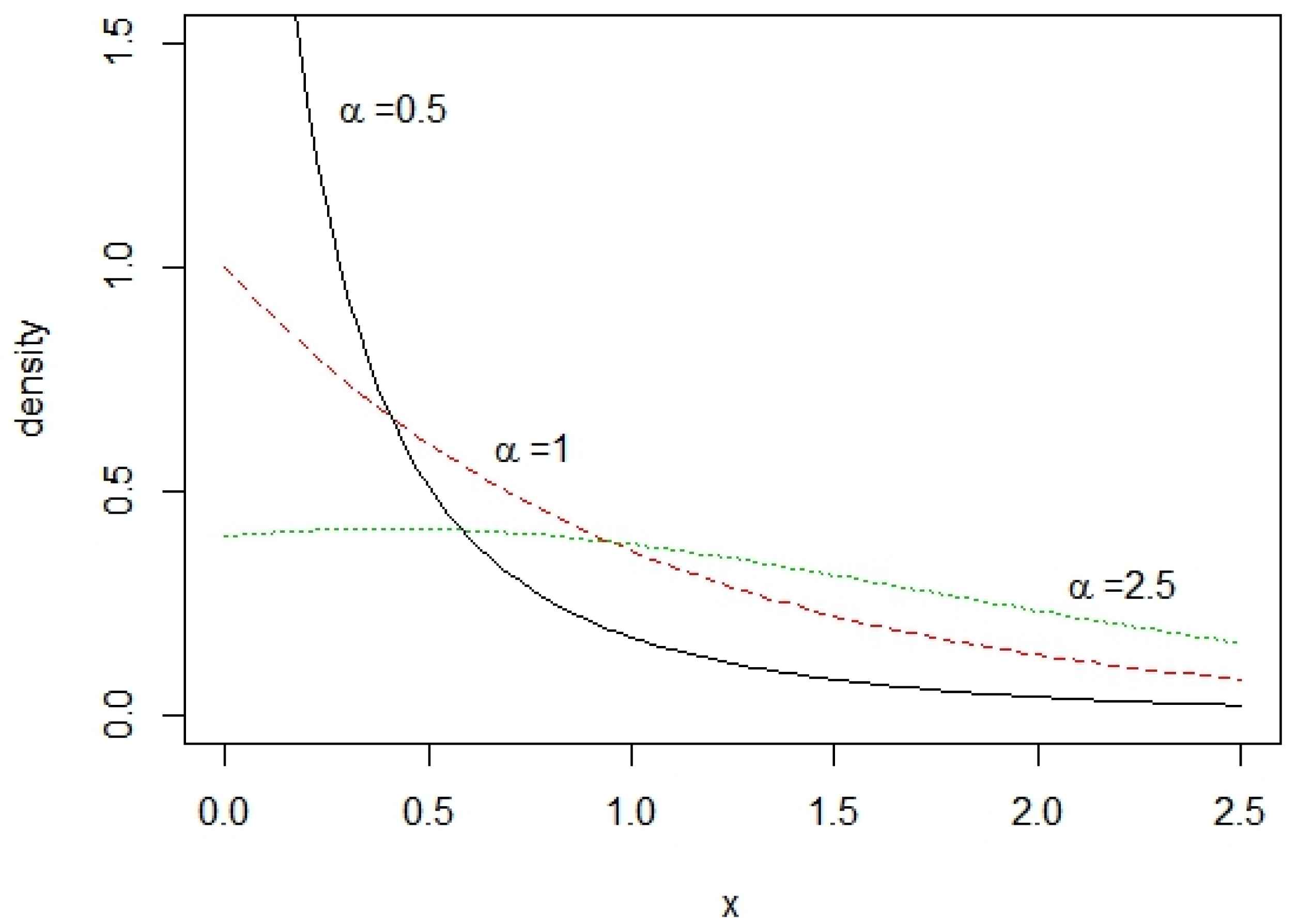
It is presented different estimators of tilt parameter that discussed in previous sections. In this section we compare the performance of these estimators by using Monte Carlo simulations. The biases and root mean square errors (RMSEs) of different estimators of α and λ in a Marshall-Olkin extended exponential distribution are presented in Table 1. These criteria were computed by simulating samples of size n = 10 and 30, each sample replicated 5000 times. The values of the α are 0.25; 1 and 2.5. In all cases we take λ = 1. The different shapes of density of MOEE(α, λ) are shown in Fig 1. We can observe that when λ is fixed, the skewness of density gets to small value with increasing α.

α	Estimators	bias		RMSE

		$αˆ$	$λˆ$	$αˆ$	$λˆ$
0.25	MLE	0.2165	0.4239	0.1898	0.5616
	MSPE	0.0056	−0.2104	0.1086	0.6506
	LSE	0.7524	−0.0020	0.8521	0.2820
	WLSE	0.0243	−0.1797	0.1292	0.7192

1	MLE	0.3232	0.1930	0.5220	0.2652
	MSPE	−0.1402	−0.2099	0.5051	0.3254
	LSE	0.0025	−0.0012	0.2889	0.2826
	WLSE	−0.0658	−0.1782	0.5572	0.3560

2.5	MLE	−0.7504	−0.0914	0.7827	0.0838
	MSPE	−1.1159	−0.2977	1.7021	0.1795
	LSE	−1.4984	0.0024	2.5261	0.2882
	WLSE	−1.0617	−0.3055	1.5987	0.1867

Table 1.

biases and RMSEs for different estimators of parameters of Marshall-Olkin Exponential when λ=1 and n=10.

From Table 1 and 2,it is observed that the MSP performs the best among all methods to estimates a for small values of a since a is a shape parameter and based on figure 1 we can see that in these cases the density is skewed. As noted before MSP method have good performance when the distribution is skewed or heavy-tailed. For estimating λ, the LS method is the best for small values of α. But when α = 2.5 the ML method is the best among all methods. In addition with increasing sample size, the performance of the MSPEs gets to the MLEs.

α	Estimators	bias		RMSE

		$αˆ$	$λˆ$	$αˆ$	$λˆ$
0.25	MLE	0.1068	0.2480	0.0581	0.3455
	MSPE	−0.0169	−0.1553	0.0386	0.3530
	LSE	0.7535	−0.0059	0.8497	0.2780
	WLSE	0.0315	−0.0249	0.0582	0.4571

1	MLE	0.2059	0.0920	0.3395	0.1210
	MSPE	−0.0893	−0.1233	0.2875	0.1309
	LSE	0.0001	0.0024	0.2878	0.2879
	WLSE	0.0577	−0.0290	0.3496	0.1478

2.5	MLE	−0.6633	−0.1020	0.5447	0.0346
	MSPE	−0.8444	−0.1892	0.9223	0.0656
	LSE	−1.5011	0.0061	2.5312	0.2869
	WLSE	−0.7684	−0.1797	0.7737	0.0596

Table 2.

biases and RMSEs for different estimators of parameters of Marshall-Olkin Exponential when λ=1 and n=30.

In table 3, For different values of sample size and α, we determined the coverage probabilities of the 90%, 95% and 99% confidence intervals for α by two methods: Confidence interval based on an asymptotic normal pivotal quantity that is obtained from (5.7) and confidence interval based on score test method that is denoted in (5.8). In all cases we assume X~MOEE(α,λ).

Sample size	α	90% CI		95% CI		99% CI
Sample size	α	ML	SC	ML	SC	ML	SC
n=10	0.25	88.39	90.71	90.94	95.35	94.42	99.09
	1	87.71	90.22	90.79	94.96	94.38	99.08
	2.5	88.06	90.58	90.32	95.10	94.72	99.15

n=30	0.25	89.80	90.39	93.43	94.89	96.89	99.20
	1	89.22	89.91	93.84	95.50	96.99	99.05
	2.5	89.45	90.11	93.33	94.77	97.08	99.07

n=50	0.25	90.20	90.38	93.94	94.97	97.95	99.12
	1	90.22	89.80	94.15	95.16	97.99	99.18
	2.5	89.94	89.83	93.88	94.88	97.72	98.95

Table 3.

Coverage probabilities (in %) of confidence interval based on maximum likelihood (ML) and score test (SC) methods for α when λ = 1.

From Table 3, it is clear that the SC confidence interval (based on score test statistic) seems to have considerably higher coverage probabilities compared to the ML confidence interval that is based on asymptotic distribution of MLE.

7. Real Data

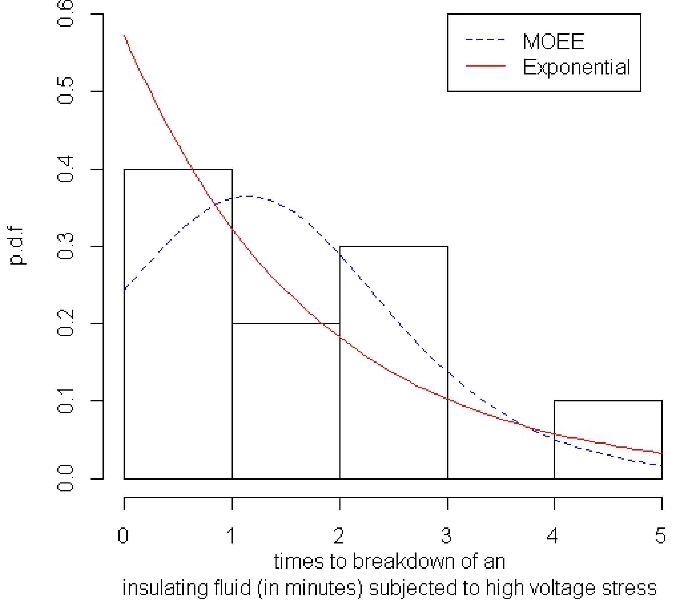
For further discussions, we analyze times to breakdown (in minutes) of an insulating fluid subjected to high voltage stress, which was reported by Ref. 12 (p. 462). We use group 3 of data for our goal.

Plots of the estimated density functions of Marshall-Olkin extended exponential and exponential models based on MLEs are given in Fig 2. It is evident that the MOEE model provides a better fit than the old model.

In Table 4, the MLEs of the model parameters and some statistics, such as negative log-likelihood and Akaike Information Criterion (AIC), are listed. From this table, the MOEE distribution has lower -2LogLik and AIC values than Exponential, and so it could be chosen as the better model. In addition the Score statistic for testing the hypothesis H₀ : α = 1 against H₁ : α ≠ 1 or equally H₀ : Exp(λ) against H₁ : MOEE(α,λ) is $33.0387 (33.0387>5.99=χ2,0.052)$ Thus the null hypothesis is rejected at 5% significant level.

	Estimates		Statistics

distribution	α	λ	−2LogLik	AIC
MOEE	4.7352	1.1510	29.1428	33.14
Exponential	1	0.5720	31.1694	33.16

Table 4.

MLEs and the measures -2LogLik and AIC

8. Conclusions

Ref. 11 proposed a simple generalization of a baseline distribution function by adding a tilt parameter α> 0 in order to obtain a larger class of distribution functions, which contains the parent distribution when α = 1. In this paper we investigated statistical inference about tilt parameter. We calculated different estimator for tilt parameter and studied their performances. Also we discussed about hypothesis testing and interval estimation of tilt parameter based on score test statistic. Finally in a real dataset, we fitted a Marshall-Olkin extended exponential and obtain MLEs of its parameters.

References

[1]S Anatolyev and G Kosenok, An alternative to maximum likelihood based on spacings, Econometric Theory, Vol. 21, 2005, pp. 472-476.

[2]Omar M Bdair, Different Methods of Estimation For Marshall Olkin Exponential Distribution, Journal of Applied Statistical Science, Vol. 19, No. 19, 2011, pp. 13-29.

[3]RCH Cheng and NAK Amin, Estimating parameters in continuous univariate distributions with a shifted origin, Journal of Royal Statistical Society. Ser. B, Vol. 45, 1983, pp. 394-403.

[4]M Ekström, Alternatives to maximum likelihood estimation based on spacings and the Kullback–Leibler divergence, Journal of Statistical Planning and Inference, Vol. 138, 2008, pp. 1778-1791.

[5]ME Ghitany, Marshall-Olkin extended Pareto distribution and its application, Int J Appl Math, Vol. 18, 2005, pp. 1732.

[6]ME Ghitany, FA Al-Awadhi, and LA Alkhalfan, Marshall-Olkin extended Lomax distribution and its application to censored data, Communications in Statistics: Theory and Methods, Vol. 36, 2007, pp. 1855-1866.

[7]R Gupta, ME Ghitany, and DK Al-Mutairi, Estimation of reliability from Marshall–Olkin extended Lomax distributions, Journal of Statistical Computation and Simulation, Vol. 80, 2010, pp. 937-947.

[8]R Gupta and C Peng, Estimating reliability in proportional odds ratio models, Computational Statistics and Data Analysis, Vol. 53, 2009, pp. 1495-1510.

[9]JHK Kao, Computer methods for estimating Weibull parameters in reliability studies, Trans. IRE-Reliability Quality Control, Vol. 13, 1958, pp. 15-22.

[10]D Kundu and M Raqab, Generalized Rayleigh distribution: different methods of estimations, Computational Statistics & Data Analysis, Vol. 49, 2005, pp. 187-200.

[11]AW Marshall and I Olkin, A new method for adding a parameter to a family of distributions with application to the exponential and Weibull families, Biometrika, Vol. 84, 1997, pp. 641-652.

[12]Wayne Nelson, Applied life data analysis, John Wiley & Sons, NY, 1982.

[13]B Ranneby, The maximum spacing method. An estimation method related to the maximum likelihood method, Scandinavian. Journal of Statistics, Vol. 11, 1984, pp. 93-112.

[14]CR Rao, Score test: historical review and recent developments, N Balakrishnan, N Kannan, and H Nagaraja (editors), Advances in ranking and selection, multiple comparisons, and reliability—methodology and applications. Statistics for industry and technology chap 1, Birkhäuser, Boston, 2005, pp. 3-20.

[15]MM Ristic, KK Jose, and J Ancy, A Marshall- Olkin gamma distribution and minification process, Stress Anxiety Res Soc, Vol. 11, 2007, pp. 107-117.

[16]J J. Swain, S Venkatraman, and J Wilson, Least-squares estimation of distribution function in Johnson’s translation system, Journal of Statistical Computation and Simulation, Vol. 29, 1988, pp. 271-297.

<Previous Article In Issue

Download article (PDF)

Next Article In Issue>

Journal: Journal of Statistical Theory and Applications
Volume-Issue: 17 - 2
Pages: 261 - 270
Publication Date: 2018/06/30
ISSN (Online): 2214-1766
ISSN (Print): 1538-7887
DOI: 10.2991/jsta.2018.17.2.6 How to use a DOI?
Open Access: This is an open access article under the CC BY-NC license (http://creativecommons.org/licences/by-nc/4.0/).

Cite this article

ris enw bib

TY  - JOUR
AU  - Mostafa Tamandi
PY  - 2018
DA  - 2018/06/30
TI  - On Inference about Tilt Parameter in Marshall-Olkin Family of Distributions
JO  - Journal of Statistical Theory and Applications
SP  - 261
EP  - 270
VL  - 17
IS  - 2
SN  - 2214-1766
UR  - https://doi.org/10.2991/jsta.2018.17.2.6
DO  - 10.2991/jsta.2018.17.2.6
ID  - Tamandi2018
ER  -

download .riscopy to clipboard