
Estimating the Modified Weibull Parameters in Presence of Constant-Stress Partially Accelerated Life Testing
- DOI
- 10.2991/jsta.2018.17.2.5How to use a DOI?
- Keywords
- Modified Weilbull distribution; Constant-partially accelerated life testing; Progressive Type-II censoring; Asymptotic confidence intervals; Bootstrap; Bayesian estimation
- Abstract
Accelerated life testing is very important in life testing experiments because it saves time and cost. In this paper, assuming that the lifetime of items under use condition follows the modified Weilbull distribution, partially accelerated life tests based on progressive Type-II censored samples are considered. The likelihood equations are to be solved numerically to obtain the maximum likelihood estimates. Based on normal approximation to the asymptotic distribution of maximum likelihood estimates, the approximate confidence intervals for the parameters are derived. Two bootstrap confidence intervals called bootstrap-p and bootstrap-t are also discussed. It is difficult to get explicit form for Bayes estimates, so we use Markov chain Monte Carlo method to solve this problem, which gives us flexibility to construct the credible intervals for parameters. Finally, a simulation study is performed to compare between MLEs and Bayes estimates.
- Copyright
- Copyright © 2018, the Authors. Published by Atlantis Press.
- Open Access
- This is an open access article under the CC BY-NC license (http://creativecommons.org/licences/by-nc/4.0/).
- ALT
Accelerated Life Test
- PALT
Partially ALT
- C-SPALT
Constant-stress PALT
- SF
Reliability Function
- HRF
Hazard Rate Function
- BP
Percentile Bootstrap
- BT
Bootstrap-t
- CRIs
credible intervals
- PRO-II-C
Progressive Type-II Censored
- MCMC
Markov chain Monte Carlo
- MWD
Modified Weilbull Distribution
Probability Density Function
- CDF
Cumulative Distribution Function
- MLEs
Maximum Likelihood Estimates
- ACIs
Approximate Confidence Intervals
- M-H
Metropolis-Hastings method
1. Introduction
There is a difficulity in getting information about the lifetime of products with high quality during testing under normal conditions, so ALTs are used in manufacturing industries to get failure data in short period of time. According to Nelson [24] there exist three ALT methods. The first one is called constant-stress ALT, where the stress is being constant during the experiment [3, 5, 4, 18]. The second one is called progressive-stress ALT, where the applied stress is increasing during time [6, 31]. The third one is called step-stress ALT,where the test condition changes at a certain time or after the termination of specific number of failures. Miler and Nelson [23] got the optimal step-stress ALT plans in the case where tested items have exponentially distributed lives and are observed until all tests fail. For more researches on ALTs, see others [14, 17, 20, 25, 28, 32]. In ALTs, the test items are tested at accelerated conditions, by applying higher levels of stress, to induce failures. Data collected at such accelerated conditions are then extrapolated through statistical model to estimate the lifetime distribution at normal condition. We use PALT when the acceleration factor is unknown, where items are examined at both normal and accelerated conditions. The stress in PALT can be divided into 3-types which are constant-stress, step-stress and progressive-stress. In step-stress PALT, items are tested at normal level, then the stress will be changed at a certain time. Many authers have dealt with this type, including Abdel-Hamid and Al-Hussaini [2].In C-SPALT (which is the main topic of this paper) we run each item at either normal or accelerated condition only. In life testing experiments, our target is to save time and cost and this leads us to what is known as censoring in which complete data about failure times for all experimental units may not be obtained, but data obtained from these experiments are called censored data. The most common censoring schemes are Type-I censoring and Type-II censoring, but in these two types the withdrawing of units is not allowed until the end of the experiment, so a more general censoring scheme called PRO-II-C has been used in this paper to overcome this problem in which the removal of prespecified number of units is done when an individual unit fails, this continues until fixed number of units fail, at which stage the remainder of the surviving units are removed. Another generalization of Weibull distribution called MWD was introduced by Xie et al. [33] and a detailed statistical analysis was given in Tang et al. [29]. The distribution is in fact a generalization of the model studied by Chen [9]. If X follows a MWD, then the PDF, CDF, SF and HRF are given respectively by
The shape of h1 (x) of MWD depends only on the shape parameter α, see [19].
- •
For α ≥ 1: h1 (x) is an increasing function.
- •
For 0 < α < 1: h1 (x) is decreasing for
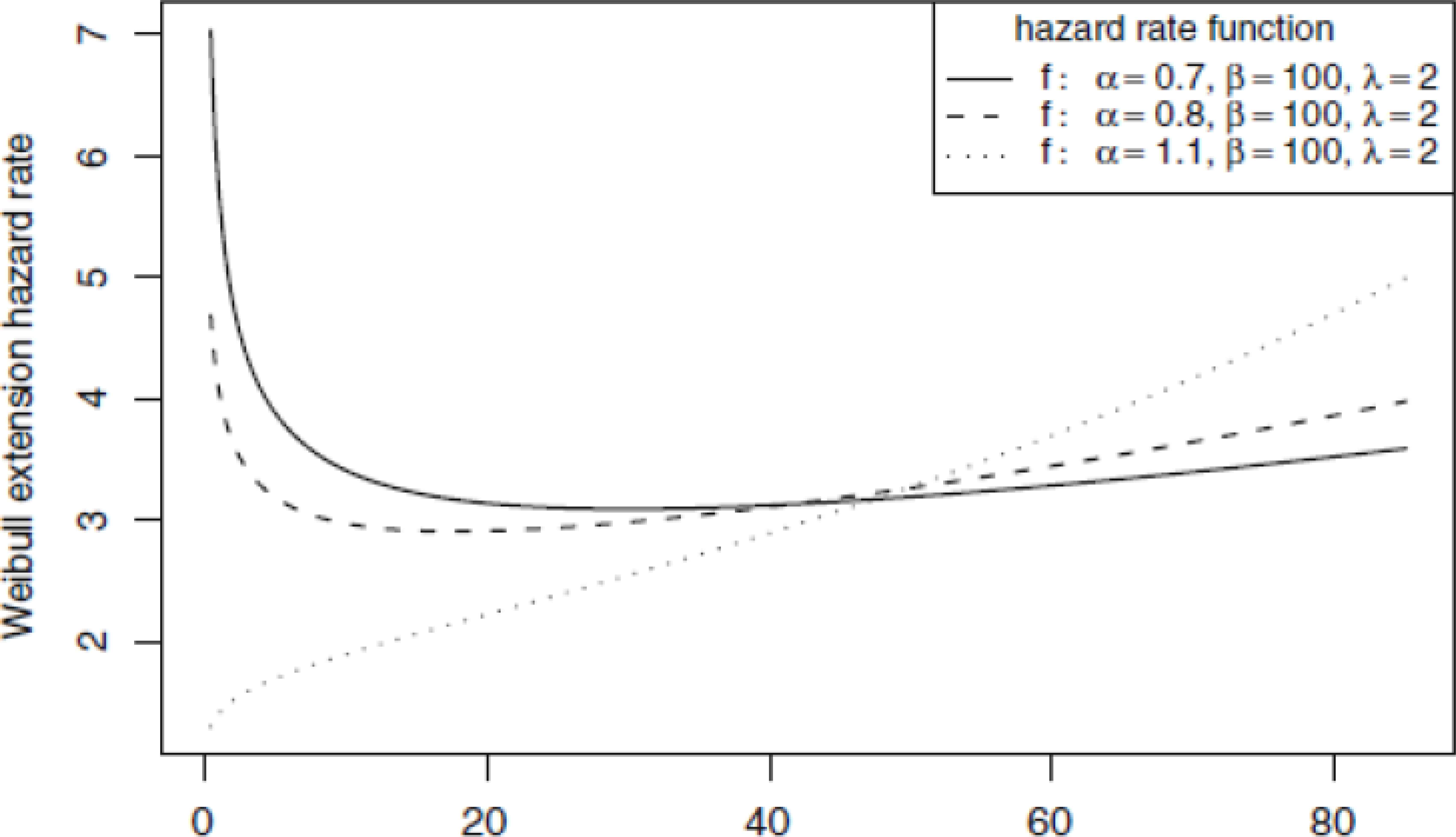
Weibull extension hazard rate functions
It is clear that the exponential power distribution(α,β) is a special case of MWD with λ = 1, so any results obtained in our study, will also be valid for the exponential Power distribution(α,β) and this was considered and studied by Smith and Bain [27].The MWD model has been fitted to the failure times of Aarset data (Aarset [1]) and the failure times of a sample of devices in a large system Gupta et al. [15].The detailed description of the data set can be found in Meeker and Escobar [21].
This paper can be organized as follows: In Section 2 some basic assumptions and description of the model are presented. The derivation of the MLEs of the parameters as well as the corresponding ACIs and the two parametric bootstrap confidence intervals for the parameters are showed in Section 3. Section 4 discusses the Bayesian approach that uses the well-known MCMC method. A numerical example to depict the approach is given in Section 5. A simulation study is presented in Section 6. Finally, some concluding remarks are considered in Section 7.
2. Model description and assumptions
In C-SPALT, n1 items are randomly selected among n test items and tested under use condition and n2 = n − n1 remaining items are subjected to an accelerated condition. PRO-II-C is applied as follows, when the first failure occurs,
Now, we assume that the lifetime of the items tested at use condition follows a MWD with PDF,CDF,SF and HRF given in (1.1)–(1.4). The hazard rate of an item tested at accelerated condition is given by h2 (x) = μh1 (x), where μ is an acceleration factor satisfying μ > 1. Therefore, the HRF, SF, CDF and PDF under acceerated condition are given respectively by
3. Maximum likelihood estimation
Let
Therefore, the log-likelihood function
Then, we differentiate (3.3) with respect to α, β,λ and μ and equate each result to zero. For simplification, we can write
A system of nonlinear simultaneous equations in four unknowns vaiables α, β, λ and μ is resulted, but it is not an easy task to get an exact solution, so we tackle this situation by using a numerical method such as Newton-Raphson to obtain an approximate solution of the above nonlinear system, see EL-Sagheer [13].
3.1. Approximate interval estimation
Upon forming the Fisher information matrix, we take the inverse of it to get the asymptotic variances and covariances of the MLE for parameters α, β, λ and μ, but unfortunately, the exact mathematical expressions are very difficult to obtain, so we give an approximate asymptotic varaince-covariance matrix for the MLE by ignoring the expectation operator E.
The common method to construct the confidence interval for the parameters α, β, λ and μ is to use the asymptotic normal distribution of MLEs and this is showed by Vander Weil and Meeker [30]. Therefore, (1 − γ)100% confidence intervals for parameters α, β, λ and μ become
3.2. Bootstrap confidence intervals
The bootstrap is a resampling method for statistical inference and commonly used to estimate CIs. For more information about parametric and non-parametric bootstrap methods, see [10, 12]. We propose to use confidence intervals based on the parameteric bootstrap methods (i) BP method based on the idea of Efron [11], (ii) BT method based on the idea of Hall [16]. The algorithms for estimating the confidence intervals using both methods are illustrated below.
3.2.1. BP method
- Step1:
From the original data
- Step2:
Use
- Step3:
As in Step 1, based on
- Step4:
Repeat Steps 2–3 N times representing N bootstrap MLE’s of α, β, λ and μ based on N different bootstrap samples.
- Step5:
Arrange all
Let
3.2.2. BT method
- Step 1:
From the original data
- Step 2:
Using
where - Step 3:
Repeat Step 2, N boot times.
For the
The 100(1 − γ)% ACI of
4. Bayesian estimation using MCMC
In this section we describe how to obtain the Bayes estimates and the corresponding credible intervals of parameters α, β, λ and μ when they are unknown. In some situations where we do not have sufficient prior information, we can use non-informative uniform distribution as the prior distribution. . The joint posterior density will then be in proportion to the likelihood function. Here we consider the prior distributions for our parameters α, β, λ and μ are
Therefore, the joint prior of the four parameters can be expressed by
The joint posterior density function of α, β, λ and μ given the data, denoted by
It is not possible to compute (4.2) analytically. Therefore, we propose the MCMC technique to generate samples from the posterior distributions and then compute the Bayes estimate for each individual parameter. There are many MCMC schemes and it is difficult to choose among them, but an important sub-class of MCMC methods are Gibbs sampling and more general Metropolis-within-Gibbs sampler.
4.1. The Metropolis-Hastings -Within-Gibbs sampling
We propose to use Gibbs sampling procedure to generate a sample from the posterior density function π*(α, β, λ,μ|x) and in turn compute the Bayes estimates and also construct the corresponding credible intervals based on the generated posterior sample. In order to use the method of MCMC for estimating the parameters, namely, α, β, λ and μ, let us consider independent priors (4.1) for the parameters α, β, λ and μ. The expression for the posterior is directly proportional to the likelihood and the prior and this can be written as
The conditional posterior densities of λ, μ, α and β are as follows:
We note that Equations (4.4) and (4.5) follow gamma distribution, so samples of λ and μ can be easily generated using any gamma generating routine. The posterior of α in Equation (4.6) and the posterior of β in Equation (4.7) are unknown, but if we plot each of them, their graphs are similar to normal distribution, see Figures 3 and 4, so we use the Metropolis-Hastings (M-H) method with normal proposal distribution to generate from each of them. For more details about M-H algorithm, see [22] and [26].
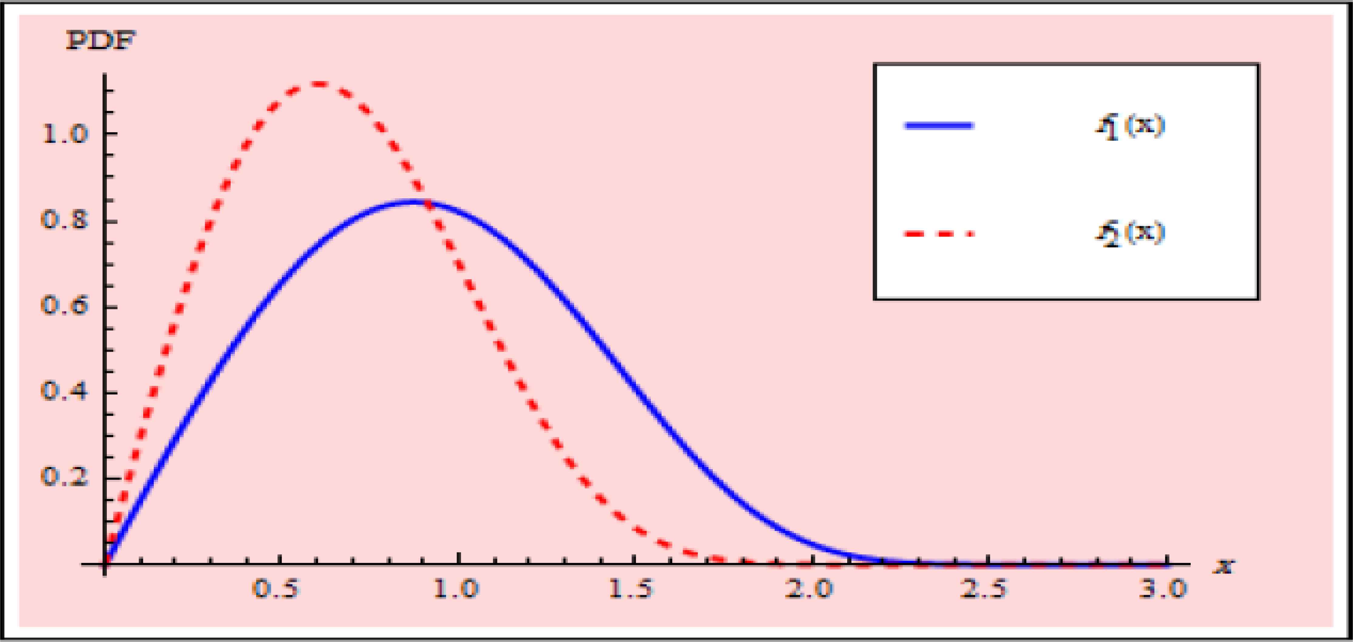
PDFs under normal and accelerated conditions
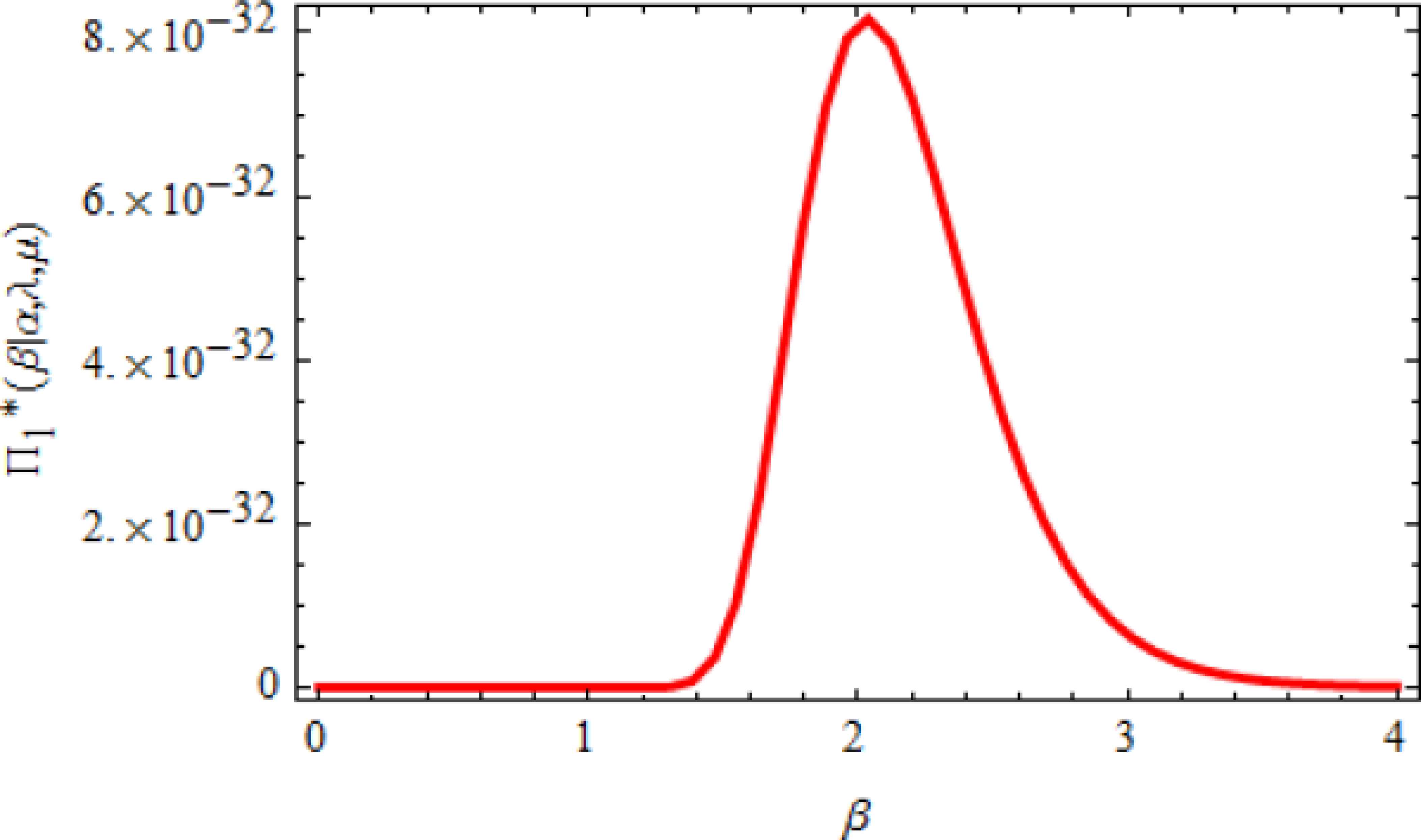
Posterior density function of β
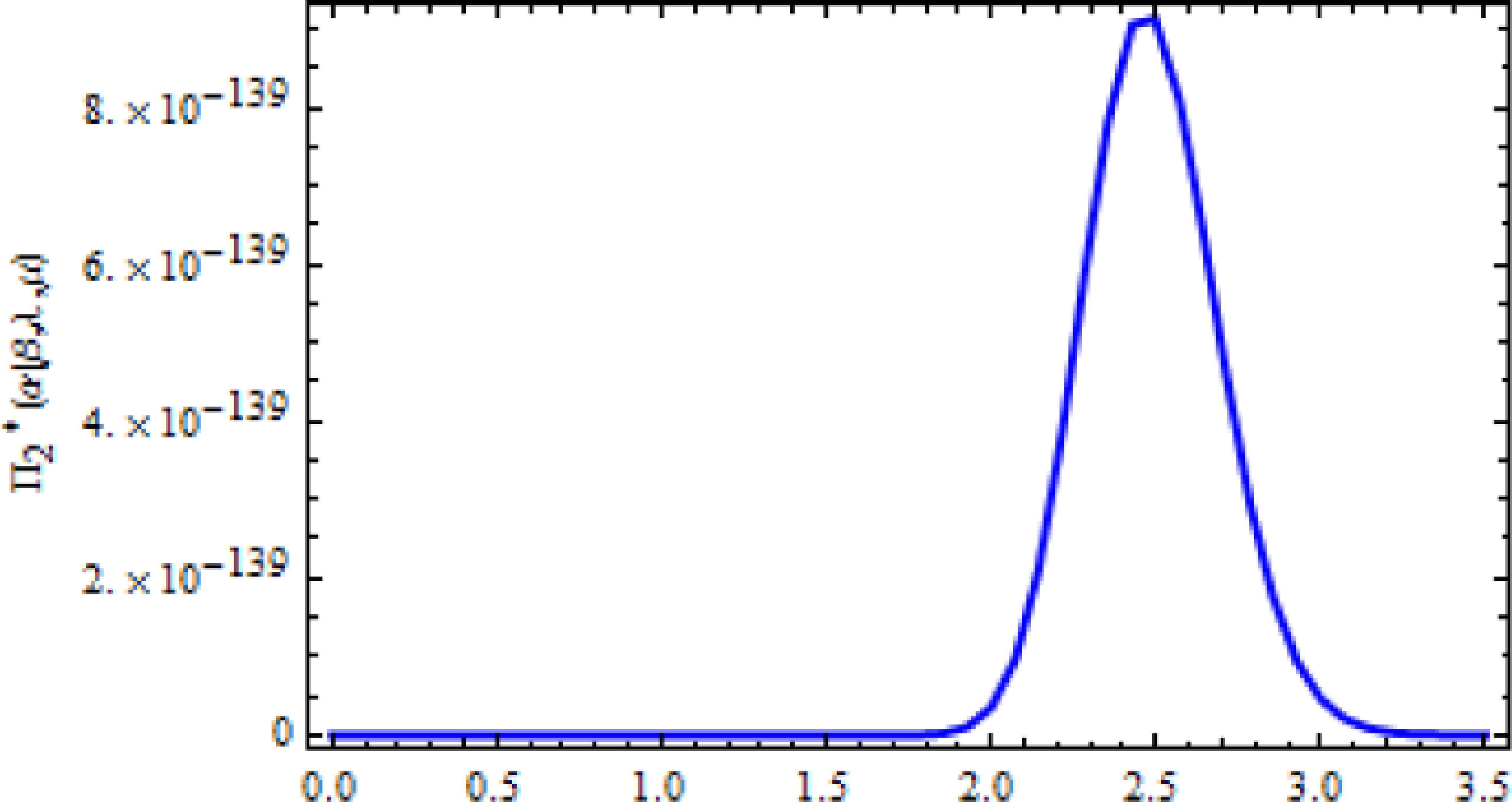
Posterior density function of α
The algorithm of Gibbs sampling is as follows:
- Step 1:
Start with an
- Step 2:
Set t = 1.
- Step 3:
Generate λ(t) from
- Step 4:
Generate μ(t) from
- Step 5:
Using M-H method, generate α(t) from
- Step 6:
Using M-H method, generate β(t) from
- Step 7:
Compute α(t), β(t), λ(t) and μ(t).
- Step 8:
Set t = t + 1.
- Step 9:
Repeat Steps 3 − 6 N times.
- Step 10:
Obtain the Bayes MCMC point estimate of ηj where η1 = α, η2 = β, η3 = λ and η4 = μ for j = 1,2,3 and 4 as
where M is the burn-in period. - Step 11:
To compute CRIs of ηj, order
5. Data analysis
In this section, we show a numerical example to check estimation procedures. We generate two samples from the modified weilbull distribution with parameters (α, β, λ, μ) = (10, 0.06, 2, 2) using progressive type-II censoring scheme with R1= (3, 1, 1, 2, 2, 1, 3, 0, 1, 5, 2, 2, 2, 1, 1, 2, 1, 0, 0, 0), R2 = (2, 0, 2, 0, 2, 0, 2, 0, 2, 0, 0, 0, 2, 0, 0, 3, 0, 1, 0, 1, 0, 1, 0, 0, 2, 0, 0, 0, 0, 0), m1 = 20, m2 = 30 and n1 = n2 = 50. The MLEs, bootstrap and bayes point estimates have been calculated for the parameters α, β, λ and μ and listed in Table 1. Also we computed 95% ACI, PBCIs, BTCIs and CRIs for the parameters and listed them in Tables 2 and 3. In MCMC procedure, the chain has been run 12000 and the first 2000 have been canceled as burn-in. Figure 1 shows the PDFs under normal and accelerated conditions.
| Parameter | ML | BP | BT | MCMC |
|---|---|---|---|---|
| α | 10.6137 | 10.0452 | 11.1165 | 11.0597 |
| β | 0.0591 | 0.0579 | 0.0602 | 0.0604 |
| λ | 1.9059 | 1.9693 | 1.8338 | 1.8501 |
| μ | 2.7211 | 2.7930 | 2.2309 | 2.1600 |
Point estimates for parameters (α, β, λ, μ) = (10, 0.06, 2, 2).
| Method | α | Length | β | Length |
|---|---|---|---|---|
| ACI | [−13.125,34.3524] | 47.4774 | [0.0323,0.0859] | 0.0536 |
| BPCI | [5.8844,11.8860] | 6.0017 | [0.0490,0.1009] | 0.0519 |
| BTCI | [5.6916,14.6896] | 8.9980 | [0.0351,0.0862] | 0.0511 |
| CRI | [4.3584,13.0047] | 8.6463 | [0.0302,0.0774] | 0.0472 |
95% Confidence intervals for parameters α and β.
| Method | λ | Length | μ | Length |
|---|---|---|---|---|
| ACI | [−8.5964, 11.4082] | 20.0047 | [1.1039, 4.3383] | 3.2345 |
| BPCI | [0.1319, 2.7786] | 2.6466 | [1.4858, 4.4691] | 2.9833 |
| BTCI | [0.1121, 3.5866] | 3.4745 | [0.0532, 2.8848] | 2.8315 |
| CRI | [1.4251, 3.0219] | 1.5968 | [1.6561, 4.4182] | 2.7621 |
95% Confidence intervals for parameters λ and μ.
6. Numerical comparison
In this section, we made a simulation study using MATHEMATICA ver. 8.0 and computed the average point estimates (AVG) and the mean square error (MSE) for the parameters α, β, λ and μ. The procedure was performed 1000 times and the population parameters were (α,β,λ, μ) =(10, 0.06, 2, 2) with sample sizes n1 = n2 = n and m1 = m2 = m and results are shown in Table 4.
| (n,m) | CS | MLE | MCMC | ||||||
|---|---|---|---|---|---|---|---|---|---|
| α | β | λ | μ | α | β | λ | μ | ||
| (30,15) | I | 9.261 (0.545) |
0.059 (0.000005) |
1.953 (0.002) |
1.699 (0.09) |
8.908 (1.191) |
0.058 (0.000005) |
2.117 (0.013) |
1.846 (0.023) |
| II | 10.149 (0.562) |
0.059 (0.0011) |
1.644 (0.295) |
2.327 (0.513) |
8.257 (4.118) |
0.059 (0.0097) |
2.277 (0.82) |
1.988 (0.083) |
|
| III | 10.396 (0.694) |
0.059 (0.008) |
1.741 (0.418) |
2.483 (0.687) |
7.531 (9.942) |
0.059 (0.009) |
3.14 (2.47) |
1.907 (0.126) |
|
| (30,25) | I | 10.269 (0.522) |
0.059 (0.006) |
1.830 (0.263) |
2.215 (0.32) |
9.465 (0.962) |
0.059 (0.006) |
2.237 (0.45) |
2.138 (0.213) |
| II | 10.211 (0.636) |
0.059 (0.008) |
1.682 (0.309) |
2.33 (0.413) |
9.060 (1.481) |
0.058 (0.008) |
2.243 (0.466) |
2.140 (0.182) |
|
| III | 10.234 (0.636) |
0.059 (0.008) |
1.814 (0.234) |
2.299 (0.317) |
8.697 (2.784) |
0.058 (0.008) |
2.529 (0.723) |
2.021 (0.064) |
|
| (50,25) | I | 10.336 (0.709) |
0.059 (0.008) |
1.751 (0.321) |
2.293 (0.416) |
9.356 (1.103) |
0.059 (0.008) |
2.233 (0.552) |
2.153 (0.181) |
| II | 10.144 (0.562) |
0.059 (0.001) |
1.618 (0.255) |
2.272 (0.326) |
8.576 (3.156) |
0.059 (0.001) |
2.201 (0.323) |
2.001 (0.093) |
|
| III | 10.362 (0.704) |
0.059 (0.007) |
1.791 (0.423) |
2.372 (0.552) |
9.156 (2.505) |
0.058 (0.0076) |
2.377 (0.970) |
2.143 (0.179) |
|
| (50,40) | I | 10.178 (0.620) |
0.058 (0.008) |
1.814 (0.342) |
2.234 (0.266) |
9.723 (1.421) |
0.0589 (0.008) |
2.036 (0.705) |
2.222 (0.235) |
| II | 10.056 (0.426) |
0.059 (0.006) |
1.877 (0.237) |
2.183 (0.145) |
9.760 (0.405) |
0.05 (0.006) |
2.025 (0.265) |
2.189 (0.151) |
|
| III | 10.239 (0.557) |
0.059 (0.006) |
1.857 (0.207) |
2.250 (0.198) |
9.882 (0.432) |
0.058 (0.006) |
2.028 (0.202) |
2.237 (0.168) |
|
| (100,50) | I | 10.094 (0.380) |
0.059 (0.005) |
1.833 (0.243) |
2.184 (0.209) |
9.773 (0.615) |
0.0599 (0.0056) |
1.968 (0.263) |
2.196 (0.201) |
| II | 10.038 (0.407) |
0.059 (0.006) |
1.822 (0.187) |
2.176 (0.193) |
9.841 (0.380) |
0.0597 (0.006) |
1.913 (0.160) |
2.186 (0.195) |
|
| III | 10.132 (0.412) |
0.059 (0.004) |
1.817 (0.127) |
2.304 (0.267) |
9.879 (0.349) |
0.059 (0.059) |
1.932 (0.097) |
2.292 (0.230) |
|
| (100,75) | I | 10.095 (0.430) |
0.059 (0.005) |
1.860 (0.145) |
2.154 (0.098) |
10.017 (0.395) |
0.059 (0.005) |
1.892 (0.135) |
2.190 (0.124) |
| II | 10.068 (0.412) |
0.059 (0.006) |
1.893 (0.158) |
2.079 (0.103) |
9.855 (0.360) |
0.058 (0.006) |
1.975 (0.149) |
2.066 (0.093) |
|
| III | 10.081 (0.367) |
0.059 (0.005) |
1.798 (0.153) |
2.138 (0.096) |
9.998 (0.344) |
0.059 (0.005) |
1.828 (0.141) |
2.184 (0.120) |
|
AVG and MSE of ML and Bayes estimates for (α, β, λ,μ) = (10,0.06,2,2).
| at constant α = 1 | |||||||
|---|---|---|---|---|---|---|---|
| (n,m1,m2) | CS | MLE | MCMC | ||||
| β | λ | μ | β | λ | μ | ||
| (20,10,20) | I | 0.0595 (0.000039) |
2.2412 (0.175) |
1.768 (0.1137) |
0.0813 (0.000736) |
3.0334 (1.496) |
1.874 (0.0729) |
| II | 0.0634 (0.000099) |
2.398 (0.2586) |
1.711 (0.1414) |
0.0815 (0.02459) |
2.9633 (1.4942) |
1.8591 (0.1167) |
|
| III | 0.0706 (0.00049) |
2.3604 (0.2413) |
1.6939 (0.1518) |
0.2053 (0.12144) |
3.5787 (3.2679) |
1.7144 (0.1341) |
|
| (20,15,30) | I | 0.0612 (0.000079) |
2.3479 (0.212) |
1.7185 (0.141) |
0.0594 (0.02294) |
2.9502 (1.7419) |
1.7814 (0.117) |
| II | 0.0639 (0.000096) |
2.4036 (0.2523) |
1.7455 (0.1202) |
0.0662 (0.02091) |
2.9805 (1.4225) |
1.7973 (0.1003) |
|
| III | 0.0633 (0.000127) |
2.3429 (0.2425) |
1.6993 (0.1485) |
0.1016 (0.0038) |
3.1577 (1.8259) |
1.8746 (2.0778) |
|
| (40,20,40) | I | 0.0635 (0.000071) |
2.4268 (0.2902) |
1.7509 (0.1265) |
0.0495 (0.06141) |
2.8796 (1.1537) |
1.796 (0.1106) |
| II | .0625 (0.000084) |
2.3693 (0.2228) |
1.718 (0.1288) |
0.071 (0.000283) |
2.6171 (0.5426) |
1.7737 (0.1037) |
|
| III | 0.07 (0.00027) |
2.4429 (0.2714) |
1.7695 (0.1078) |
0.1848 (0.16457) |
3.1837 (1.835) |
2.1503 (5.229) |
|
| (40,30,60) | I | 0.0621 (0.000049) |
2.3523 (0.2032) |
1.7305 (0.1134) |
0.0677 (0.000127) |
2.6087 (0.4954) |
1.7623 (0.0966) |
| II | 0.0631 (0.00052) |
2.4219 (0.2576) |
1.7492 (0.0887) |
0.0689 (0.00015) |
2.6488 (0.5372) |
1.7817 (0.075) |
|
| III | 0.0656 (0.000107) |
2.4295 (0.26) |
1.7411 (0.1005) |
0.0805 (0.000823) |
2.8295 (0.8777) |
1.7528 (0.094) |
|
| (60,30,60) | I | 0.0631 (0.000045) |
2.4061 (0.2409) |
1.7402 (0.1055) |
0.0689 (0.000147) |
2.6615 (0.5708) |
1.7766 (0.0923) |
| II | 0.061 (0.0000447) |
2.2998 (0.1542) |
1.7173 (0.1222) |
0.061 (0.000117) |
2.49 (0.3257) |
1.7463 (0.1072) |
|
| III | 0.0682 (0.000181) |
2.4393 (0.2578) |
1.7343 (0.1097) |
0.0895 (0.01906) |
2.9274 (1.091) |
1.7261 (0.1126) |
|
| (60,50,90) | I | 0.0627 (0.000037) |
2.4049 (0.2314) |
1.707 (0.1114) |
0.066 (0.000081) |
2.5637 (0.4084) |
1.7263 (0.1004) |
| II | 0.0628 (0.000031) |
2.3958 (0.2098) |
1.7377 (0.0942) |
0.0662 (0.000069) |
2.5464 (0.3607) |
1.7538 (0.0875) |
|
| III | 0.0638 (0.000085) |
2.4202 (0.236) |
1.6941 (0.1139) |
0.0696 (0.00017) |
2.6355 (0.4909) |
1.7023 (0.1092) |
|
AVG and MSE of ML and Bayes estimates for (β,λ,μ) = (0.06,2,2).
| at constant α = 1 | |||||||
|---|---|---|---|---|---|---|---|
| (n,m1,m2) | CS | MLE | MCMC | ||||
| β | λ | μ | β | λ | μ | ||
| (20,10,20) | I | 0.056 (0.99) |
3.0358 (0.99) |
4.4518 (0.99) |
0.1274 (0.99) |
6.0503 (0.99) |
3.0825 (0.99) |
| II | 0.0702 (0.99) |
4.1129 (0.99) |
4.1329 (0.99) |
0.1779 (0.97) |
5.1185 (0.98) |
2.958 (0.99) |
|
| III | 0.1403 (0.99) |
3.9614 (0.99) |
4.168 (0.99) |
0.7396 (0.87) |
5.9014 (0.92) |
2.7929 (0.99) |
|
| (20,15,30) | I | 0.0549 (0.97) |
3.3785 (0.99) |
3.7315 (0.99) |
0.1089 (0.96) |
4.8809 (0.99) |
2.2876 (0.98) |
| II | 0.0579 (0.98) |
3.1825 (0.99) |
3.4239 (0.99) |
0.1203 (0.97) |
4.7176 (0.97) |
2.2906 (0.99) |
|
| III | 0.0804 (0.99) |
3.5097 (0.99) |
3.8747 (0.98) |
0.1964 (0.96) |
5.3013 (0.99) |
3.3675 (0.98) |
|
| (40,20,40) | I | 0.0579 (0.98) |
4.2019 (0.99) |
3.0721 (0.98) |
0.190 (0.99) |
4.2443 (0.99) |
1.9591 (0.99) |
| II | 0.0469 (0.97) |
2.8267 (0.98) |
2.6715 (0.99) |
0.0699 (0.98) |
3.2596 (0.96) |
1.907 (0.99) |
|
| III | 0.1017 (0.99) |
3.0864 (0.98) |
2.9879 (0.98) |
0.4108 (0.93) |
4.3802 (0.97) |
4.1805 (0.99) |
|
| (40,30,60) | I | 0.0353 (0.95) |
2.1364 (0.99) |
2.3602 (0.95) |
0.0516 (0.98) |
3.1893 (0.99) |
1.5741 (0.98) |
| II | 0.0382 (0.98) |
2.324 (0.99) |
2.3374 (0.99) |
0.0534 (0.96) |
3.0202 (0.97) |
1.5772 (0.99) |
|
| III | 0.0525 (0.99) |
2.3581 (0.98) |
2.423 (0.98) |
0.1017 (0.99) |
3.6309 (0.97) |
1.5861 (0.99) |
|
| (60,30,60) | I | 0.0384 (0.99) |
2.4577 (0.99) |
2.3284 (0.99) |
0.0521 (0.98) |
3.1558 (0.99) |
1.5741 (0.99) |
| II | 0.0426 (0.97) |
2.3196 (0.99) |
2.7185 (0.97) |
0.051 (0.99) |
2.5739 (0.98) |
1.5242 (0.99) |
|
| III | 0.0788 (0.99) |
2.4596 (0.99) |
2.4006 (0.98) |
0.2046 (0.97) |
3.4947 (0.96) |
1.5811 (0.99) |
|
| (60,50,90) | I | 0.0301 (0.95) |
1.8135 (0.99) |
1.972 (0.93) |
0.0386 (0.95) |
2.4831 (0.99) |
1.1937 (0.97) |
| II | 0.0279 (0.99) |
1.5825 (0.99) |
1.8247 (0.96) |
0.0387 (0.99) |
2.3351 (0.999) |
1.2341 (0.99) |
|
| III | 0.0328 (0.98) |
1.589 (0.96) |
1.7172 (0.95) |
0.0553 (0.96) |
2.7334 (0.98) |
1.2375 (0.96) |
|
ACL and CP of 95% CIs for (β,λ,μ) = (0.06,2,2).
| at constant β = 1 | |||||||
|---|---|---|---|---|---|---|---|
| (n,m1,m2) | CS | MLE | MCMCM | ||||
| α | λ | μ | α | λ | μ | ||
| (20,10,20) | I | 10.7008 (1.2898) |
2.501 (0.3345) |
1.8418 0.0978) |
11.0046 (1.8442) |
2.5956 (0.4541) |
2.0397 (0.1124) |
| II | 10.376 (0.7166) |
2.6447 (0.6086) |
1.6149 (0.2041) |
10.4635 (0.844) |
2.7214 (0.7559) |
1.7827 (0.1231) |
|
| III | 10.6219 (0.9651) |
3.0596 (1.4262) |
1.5332 (0.3006) |
10.8375 (1.7516) |
3.4989 (3.2126) |
1.715 (0.2077) |
|
| (20,15,30) | I | 10.3427 (0.794) |
2.2998 (0.1719) |
1.8241 (0.0891) |
10.5203 (1.0157) |
2.3462 (0.2208) |
1.9452 (0.0723) |
| II | 10.3454 (0.7494) |
2.4789 (0.341) |
1.7113 (0.1481) |
10.4634 (0.900) |
2.5291 (0.424) |
1.8254 (0.1079) |
|
| III | 10.3828 (0.7039) |
2.6167 (0.5117) |
1.657 (0.1732) |
10.5635 (1.0712) |
2.745 (0.7482) |
1.7776 (0.1213) |
|
| (40,20,40) | I | 10.3307 (0.6479) |
2.3218 (0.1802) |
1.8209 (0.0822) |
10.4596 (0.7872) |
2.3476 (0.2073) |
1.9183 (0.0674) |
| II | 10.387 (0.6155) |
2.5788 (0.4786) |
1.6489 (0.1862) |
10.4492 (0.6802) |
2.6152 (0.5303) |
1.7334 (0.1460) |
|
| III | 10.4848 (0.9172) |
2.8496 (0.9353) |
1.5301 (0.2759) |
10.6181 (1.192) |
3.033 (1.3709) |
1.6122 (0.2161) |
|
| (40,30,60) | I | 10.2877 (0.6171) |
2.2525 (0.1206) |
1.8005 (0.0765) |
10.3642 (0.7097) |
2.2696 (0.1349) |
1.8594 (0.0621) |
| II | 10.4576 (0.8037) |
2.445 (0.2925) |
1.7121 (0.1167) |
10.5141 (0.8842) |
2.4645 (0.3259) |
1.771 (0.0906) |
|
| III | 10.3383 (0.5735) |
2.3375 (0.1707) |
1.7607 (0.0881) |
10.436 (0.6961) |
2.3857 (0.223) |
1.8082 (0.0706) |
|
| (60,30,60) | I | 10.1902 (0.5777) |
2.2849 (0.1403) |
1.8004 (0.0811) |
10.2894 (0.6584) |
2.3057 (0.1588) |
1.8637 (0.0662) |
| II | 10.2647 (0.4723) |
2.5227 (0.3675) |
1.6399 (0.1619) |
10.3048 (0.4974) |
2.5475 (0.405) |
1.6921 (0.1292) |
|
| III | 10.2817 (0.6363) |
2.3968 (0.2158) |
1.746 (0.1016) |
10.3032 (0.6973) |
2.4313 (0.2794) |
1.8091 (0.0766) |
|
| (60,50,90) | I | 10.1694 (0.5023) |
2024 (0.0986) |
1.8155 (0.0697) |
10.2176 (0.5666) |
2.2495 (0.1082) |
1.853 (0.0609) |
| II | 10.1431 (0.4156) |
2.2866 (0.1393) |
1.7472 (0.0873) |
10.1724 (0.4323) |
2.2966 (0.1486) |
1.7797 (0.0734) |
|
| III | 10.4057 (0.7198) |
2.3178 (0.152) |
1.7909 (0.0785) |
10.4669 (0.7897) |
2.3402 (0.1711) |
1.8256 (0.0694) |
|
AVG and MSE of ML and Bayes estimates for (α,λ, μ) =(10,2,2).
| at constant β = 1 | |||||||
|---|---|---|---|---|---|---|---|
| (n,m1,m2) | CS | MLE | MCMC | ||||
| α | λ | μ | α | λ | μ | ||
| (20,10,20) | I | 11.1008 (0.99) |
5.3223 (0.99) |
3.9355 (0.99) |
9.0397 (0.99) |
3.7072 (0.99) |
3.2527 (0.99) |
| II | 6.7916 (0.99) |
4.2454 (0.99) |
3.6891 (0.98) |
7.6956 (0.97) |
4.183 (0.99) |
2.8243 (0.99) |
|
| III | 6.0575 (0.99) |
5.1354 (0.98) |
3.7134 (0.98) |
9.7149 (0.99) |
7.8724 (0.995) |
2.7028 (0.993) |
|
| (20,15,30) | I | 9.9457 (0.992) |
3.3441 (0.994) |
3.6462 (0.995) |
7.1839 (0.991) |
2.555 (0.998) |
2.4516 (0.996) |
| II | 7.5563 (0.998) |
3.6064 (0.99) |
3.1659 (0.997) |
6.9438 (0.999) |
2.9543 (0.995) |
2.2971 (0.991) |
|
| III | 6.9475 (0.999) |
3.5343 (0.996) |
3.1699 (0.993) |
7.9778 (0.995) |
3.774 (0.994) |
2.2567 (0.999) |
|
| (40,20,40) | I | 6.8394 (0.99) |
2.559 (0.99) |
2.7329 (0.99) |
5.7899 (0.99) |
2.2057 (0.99) |
2.0694 (0.99) |
| II | 4.9991 (0.98) |
2.9631 (0.99) |
2.9531 (0.96) |
5.4599 (0.98) |
2.7755 (0.99) |
1.8767 (0.98) |
|
| III | 4.922 (0.92) |
3.436 (0.99) |
3.0587 (0.89) |
6.8644 (0.99) |
4.4326 (0.98) |
1.7545 (0.94) |
|
| (40,30,60) | I | 6.8264 (0.99) |
2.2883 (0.98) |
2.4979 (0.97) |
4.989 (0.99) |
1.7294 (0.99) |
1.6202 (0.99) |
| II | 5.1768 (0.98) |
2.345 (0.99) |
2.2533 (0.99) |
4.8322 (0.98) |
2.0064 (0.99) |
1.5289 (0.99) |
|
| III | 7.6706 (0.99) |
2.6993 (0.99) |
2.4883 (0.99) |
5.3526 (0.98) |
2.1018 (0.99) |
1.5218 (0.98) |
|
| (60,30,60) | I | 6.5778 (0.99) |
2.4444 (0.99) |
2.5063 (0.98) |
4.7873 (0.97) |
1.7859 (0.99) |
1.6208 (0.99) |
| II | 3.8321 (0.98) |
2.2191 (0.99) |
2.2521 (0.98) |
4.3144 (0.99) |
2.1903 (0.97) |
1.4579 (0.98) |
|
| III | 6.472 (0.99) |
2.4208 (0.99) |
2.8273 (0.99) |
5.0385 (0.98) |
2.5281 (0.97) |
1.5586 (0.99) |
|
| (60,50,90) | I | 5.7573 (0.99) |
1.6062 (0.99) |
2.3605 (0.98) |
3.9548 (0.99) |
1.3452 (0.98) |
1.2847 (0.99) |
| II | 4.6031 (0.99) |
1.5695 (0.97) |
2.2536 (0.98) |
3.7996 (0.99) |
1.4078 (0.95) |
1.228 (0.98) |
|
| III | 5.6451 (0.99) |
1.644 (0.99) |
2.0888 (0.98) |
4.2791 (0.99) |
1.550 (0.98) |
1.2402 (0.97) |
|
ACL and CP of 95% CIs for the parameters (α,λ, μ) =(10,2,2)
7. Concluding remarks
In this paper, we considered the maximun likelihood, bootstrap and Bayes estimats for the parameters of the MWD. This paper also studied the construction of confidence intervals for the parameters. We use MCMC method because we donot get explicit form for the Bayes estimate. A numerical example using simulated data is presented to show how the MCMC and parametric bootstrap methods work based on PRO-II-C. Finally, a simulation study was performed to compare the performance of MLE and Bayes estimates for different sample sizes. The following conclusions can be drawn from Tables 4, 5, 6, 7 and 8:
- (i)
From Table 4, we notice that Scheme I is the best in the sense of having smaller MSEs for fixed values of n,m1,m2.
- (ii)
From Table 5, we observe that at constant α, MLEs have smaller MSE than Bayes estimates.
- (iii)
It is observed from Table 7 that when the sample size increases, the MSEs decreases.
- (iv)
From Table 7, it can be seen that for parameters α and λ, MLEs gives more accurate results then Bayes estimates in the sense of having smaller MSEs, but for the parameter μ, Bayes estimates are better in MSEs than MLEs.
- (v)
From Table 8, it can be seen that CRIs show more accurate results than the ACIs because the lengths of CRIs are less than the lengths of ACIs.
Acknowledgement
The authors are grateful to the anonymous referee for a careful checking of the details and for helpful comments that improved this paper.
References
Cite this article
TY  - JOUR
AU  - Mohamed A. W. Mahmoud
AU  - Rashad M. EL-Sagheer
AU  - Amr M. Abou-Senna
PY  - 2018
DA  - 2018/06/30
TI  - Estimating the Modified Weibull Parameters in Presence of Constant-Stress Partially Accelerated Life Testing
JO  - Journal of Statistical Theory and Applications
SP  - 242
EP  - 260
VL  - 17
IS  - 2
SN  - 2214-1766
UR  - https://doi.org/10.2991/jsta.2018.17.2.5
DO  - 10.2991/jsta.2018.17.2.5
ID  - Mahmoud2018
ER  -