
Estimating the parameters of Lomax distribution from imprecise information
- DOI
- 10.2991/jsta.2018.17.1.9How to use a DOI?
- Keywords
- Imprecise data; Fuzzy information; Lomax distribution; Maximum likelihood estimation; Bayesian estimation
- Abstract
Traditional statistical approaches for estimating the parameters of Lomax distribution have dealt with precise information. However, in real world situations, some information about an underlying system might be imprecise and are represented in the form of fuzzy information. In this paper, we consider the problem of estimating the parameters of Lomax distribution when the available observations are described by means of fuzzy information. We obtain the maximum likelihood estimate of the parameters by using the Newton-Raphson as well as the EM algorithm. We also provide an approximation namely, Tierney and Kadane’s approximation, to compute the Bayes estimates of the unknown parameters. The estimation procedures are discussed in details and compared via Monte Carlo simulations in terms of their estimated biases and mean squared errors. Finally, analysis of one data set is provided for the purpose of illustration.
- Copyright
- Copyright © 2018, the Authors. Published by Atlantis Press.
- Open Access
- This is an open access article under the CC BY-NC license (http://creativecommons.org/licences/by-nc/4.0/).
1. Introduction
A random variable X is said to have Lomax distribution, if its probability density function (pdf) and cumulative distribution function are given, respectively, by
Lomax distribution provides a very good alternative to the common lifetime distributions such as exponential, Weibull, or gamma when the experimenter presumes that the population distribution may be heavy-tailed (see Bryson [7]). Also, it has been shown that its utilities for modeling and analyzing lifetime data in medical and biological sciences, engineering, etc. So, it has been received greatest attention from theoretical and statisticians primarily due to its use in lifetime testing studies. The Lomax distribution has been used in the literature in a number of ways. For example, it has been extensively used for reliability modelling and life testing; see, for example, Balkema and de Haan [5]. Ahsanullah [1] studied the record values of Lomax distribution. Balakrishnan and Ahsanullah [4] introduced some recurrence relations between the moments of record values from Lomax distribution.
Several authors have addressed inferential issues for the Lomax distribution based on complete and censored samples. The order statistics from nonidentical right-truncated Lomax random variables have been studied by Childs et al. [10]. Howlader and Hossain [15] considered Bayesian estimation of the survival function of the Lomax distribution. Ghitany et al. [13] considered Marshall-Olkin approach and extended Lomax distribution. Elfattah et al. [12] derived the Bayesian and the non-Baysian estimators for the same sample size from the Lomax distribution based on the progressive type-I censoring. Raqab et al. [26] discussed different predictors of failure times such as best linear unbiased predictors, and maximum-likelihood and approximate maximum-likelihood predictors based on multistage progressive censoring from Pareto distribution, and recently Cramer and Schmiedt [11] discussed the optimal censoring scheme for estimating the parameters of the Lomax distribution using progressive type-II censoring. Asgharzadeh and Valiollahi [3] derived the Bayesian estimator of the scale parameter of the Lomax distribution based on progressive type-II censoring.
From the above, it is evident that all the earlier works on the estimation of the parameters of Lomax distribution have been done under the assumption of precise data. However, in real world situations, we deal with experiments whose observation does not provide exact but imprecise information. For example, the time of reaction of a person to a certain stimulus in a psychological experience can not be exactly determined, but the psychologist is able to determine it by means of the following imprecise information: ”The time of reaction is approximately 25 to 35 seconds”. To deal with the lack of precision of the data, it is necessary to incorporate fuzzy concept to statistical techniques. In recent years, many papers on generalization of classical statistical methods to analysis of fuzzy data have been published. Among others, Buckley [8] considered fuzzy systems whose performance will depend on fuzzy probability distributions and whose measures of performance can be described by fuzzy numbers. Pak et al. [23] and [24] conducted a series of studies to develop the inferential procedures for the lifetime distributions on the basis of fuzzy numbers. Maximum likelihood estimation of exponential model using type-II fuzzy censored data is considered by Khoolenjani and Shahsanaie [17]. Makhdoom et al. [21] studied Bayesian estimation of the parameter of exponential distribution under type II censoring from fuzzy data.
To our knowledge there are no reports on estimating the parameters of Lomax distribution based on fuzzy data. The main aim of this paper is to obtain the inferential procedures for the Lomax distribution when the available observations are reported by means of fuzzy information. In Section 2, we use the Newton-Raphson and the EM algorithms to determine the maximum likelihood estimates of the unknown parameters. In Section 3, we obtain the Bayes estimates of the parameters α and λ by using the approximation form of Tierney and Kadane [32] under the assumption of gamma priors. A Monte Carlo simulation study is presented in Section 4, which provides a comparison of all estimation procedures developed in this paper and analysis of a data set is provided. Finally, conclusions and recommendations are provided in Section 5.
Let us first review the fundamental notation and basic definitions of fuzzy set theory used in the paper. Consider an experiment characterized by a probability space X = (X, ℬX, Pθ), where (X, ℬX) is a measurable space and Pθ belongs to a specified family of probability measures {Pθ, θ ∈ Θ} on (X, ℬX). Assume that the observer cannot distinguish or transmit with exactness the outcome in the performance of X, but that rather the available observation may be described in terms of fuzzy information which is defined as follows:
Definition 1.
A fuzzy event
Among the various types of fuzzy information, the triangular and trapezoidal fuzzy numbers are most convenient and useful in describing fuzzy data. For triangular membership function, the triangular fuzzy number can be defined as
Definition 2.
(see Tanaka et al. [31]). A fuzzy information system (f.i.s.)
Definition 3.
The probability distribution on
2. Maximum likelihood estimation
Suppose that X1,...,Xn is a random sample of size n from Lomax distribution with pdf given by (1.1). Let X = (X1,...,Xn)denotes the corresponding random vector. If a realization x of X was known exactly, we could obtain the complete-data likelihood function as
Example 1.
A geologist is interested in analyzing the length of the largest axis of boulders in the upper reaches of a particular river. Assume that the geologist does not have a mechanism of measurement sufficiently precise to determine exactly the length of the largest axis of boulders. More precisely, suppose that the lack of roundness of these boulders only allows him to approximate the length of the largest axes by means of the following fuzzy observations:
Once
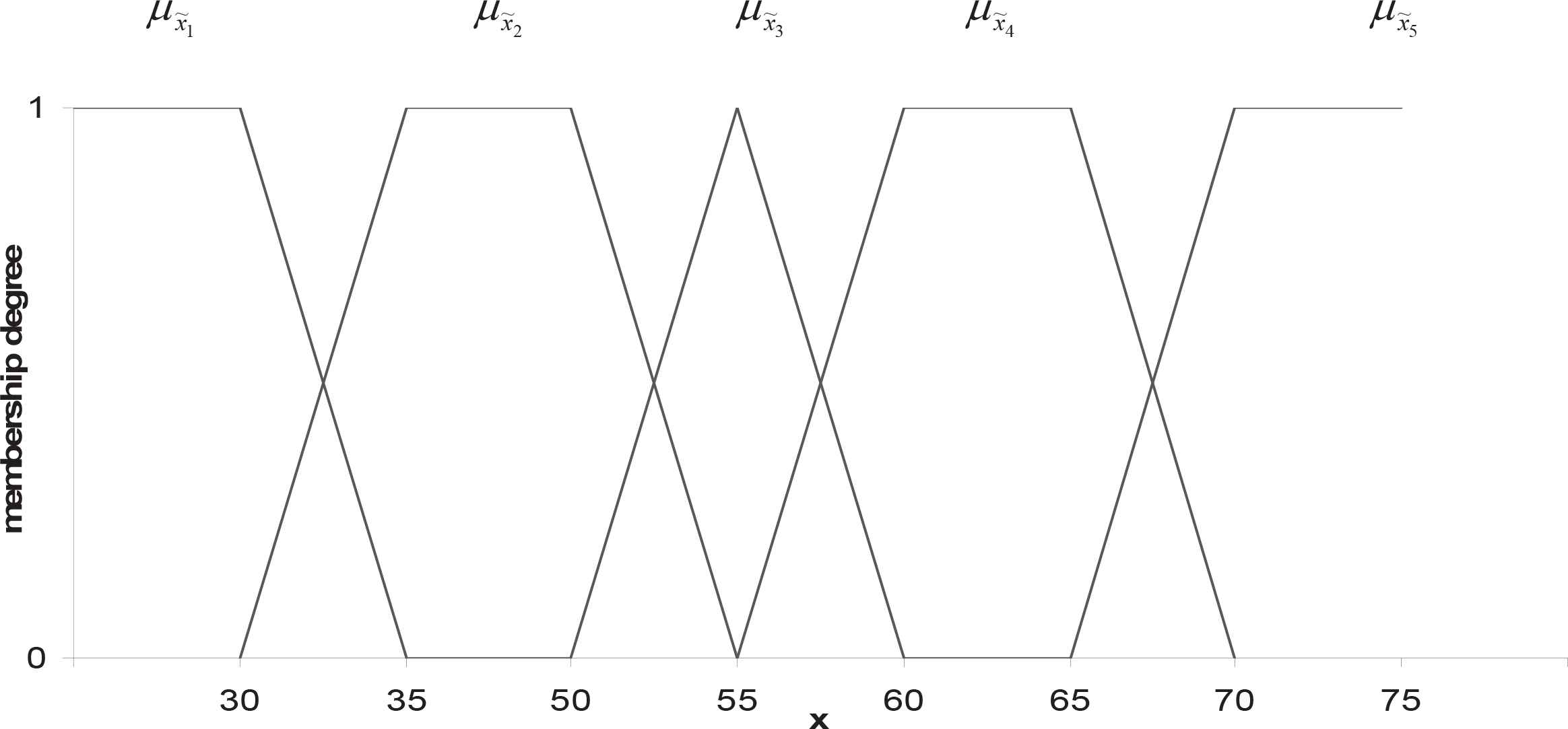
Membership functions of the fuzzy observations
2.1. Newton-Raphson algorithm
The Newton-Raphson algorithm is a direct approach for estimating the relevant parameters in a likelihood function. In this algorithm, the solution of the likelihood equation is obtained through an iterative procedure. Let θ = (α, λ)T be the parameter vector. Then, at the (h+1)th step of iteration process, the updated parameter is obtained as
It should be pointed out that the second-order derivatives of the log-likelihood are required at every iteration in the Newton-Raphson method. Sometimes the calculation of the derivatives based on fuzzy data can be rather tedious. Another viable alternative to the Newton-Raphson algorithm is the well-known EM algorithm. In the following, we discuss how that can be used to determine the MLEs in this case.
2.2. EM algorithm
The Expectation Maximization (EM) algorithm is a broadly applicable approach to the iterative computation of maximum likelihood estimates and useful in a variety of incomplete-data problems. Since the observed fuzzy data
From (2.1), the log-likelihood function for the complete data vector x becomes:
- 1.
Given starting values of α and λ, say α(0) and λ(0) and set h = 0.
- 2.
In the (h + 1)th iteration,
- (1)
The E-step requires to compute the following conditional expectations using the expression (1.5):
and the likelihood equations (2.7) and (2.8) are replaced by
- (1)
The M-step requires to solve the Eqs. (2.9) and (2.10) and obtain the next values, α(h+1) and λ(h+1), of α and λ, respectively, as follows:
- (1)
- 3.
Checking convergence, if the convergence occurs then the current α(h+1) and λ(h+1) are the maximum likelihood estimates of α and λ via EM algorithm; otherwise, set h = h + 1 and go to Step 2. The MLE of (α, λ) via EM algorithm is thereafter refereed as
3. Bayesian estimation
In recent decades, the Bayes viewpoint, as a powerful and valid alternative to traditional statistical perspectives, has received frequent attention for statistical inference. In this section, we consider the Bayesian estimation of the unknown parameters by using a squared error loss function. In order to evaluate the behavior of the parameters, it is assumed that α and λ have independent gamma priors with the pdfs
Setting H(α, λ) = Q(α, λ)/n and H* (α, λ) = [lng(α, λ) + Q(α, λ)]/n, the expression in (3.4) can be reexpressed as
In our case, we have
4. Numerical Study
4.1. Monte Carlo Simulations
In this section, we present some experimental results, mainly to observe how the different methods behave for different sample sizes. We obtain the estimates of the unknown parameters α and λ by using the methods provided in the preceding sections. The performance of the competitive estimates has been compared on the basis of their estimated biases and mean squared errors. The computations are performed using R 2.14.0 [27], which is a non-commercial, open source software package for statistical computing.
First, for two sets of parameter values namely; (α = 1, λ = 1) and (α = 2, λ = 1.5)and various choices of sample size n, we have generated i.i.d random samples from the Lomax distribution. Then, using the method proposed by Pak et al. [24], each realization of the generated samples was fuzzified by employing the fuzzy information system shown in Fig. 2, and the estimates of parameters for the fuzzy sample were computed using the maximum likelihood method (via Newton-Raphson and EM algorithms) and Bayesian procedure. To make the comparison between ML and Bayes estimates meaningful, two types of priors are suggested, namely non-informative prior and informative gamma prior (Lin et al. [19]). The first one is used when we do not have any prior information about the parameters while the informative priors are used to investigate any improvements in the performances of Bayes estimators. Here, we have considered two different choices of hyperparameters as
Prior I: (non-informative) a = b = c = d = 0
Prior II: (informative ) a = b = c = d = 2.
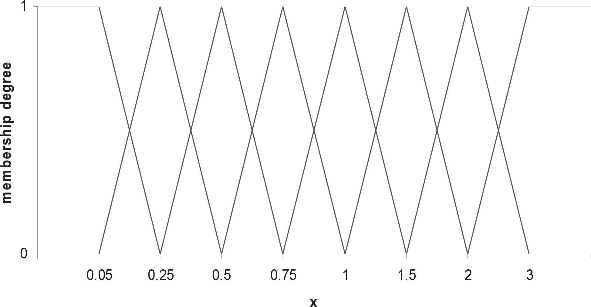
Fuzzy information system used to encode the simulated data
It must be noted that the non-informative prior I is non-proper also. Press [25] suggested to use very small non-negative values of the hyperparameters in this case, and it will make the priors proper. We have tried a = b = c = d = 0.0001. The results are not significantly different than the corresponding results obtained using non-proper priors, and are not reported due to space. From now on, the Bayes estimates of parameters obtained by using the above priors will be denoted by BET1 and BET2, respectively. The estimated biases and mean squared errors of the estimates over 1000 replications are presented in Tables 1–4.
| n | NR | EM | BET1 | BET2 | ||||
|---|---|---|---|---|---|---|---|---|
| EB | MSE | EB | MSE | EB | MSE | EB | MSE | |
| 15 | 0.0567 | 0.0396 | 0.0569 | 0.0397 | 0.0553 | 0.0391 | 0.0535 | 0.0366 |
| 20 | 0.0509 | 0.0378 | 0.0511 | 0.0380 | 0.0504 | 0.0375 | 0.0477 | 0.0332 |
| 25 | 0.0482 | 0.0341 | 0.0485 | 0.0343 | 0.0479 | 0.0338 | 0.0439 | 0.0319 |
| 30 | 0.0417 | 0.0276 | 0.0419 | 0.0277 | 0.0403 | 0.0269 | 0.0381 | 0.0253 |
| 40 | 0.0362 | 0.0219 | 0.0364 | 0.0220 | 0.0361 | 0.0217 | 0.0345 | 0.0196 |
| 50 | 0.0319 | 0.0154 | 0.0319 | 0.0154 | 0.0315 | 0.0152 | 0.0307 | 0.0122 |
| 70 | 0.0254 | 0.0117 | 0.0256 | 0.0118 | 0.0237 | 0.0114 | 0.0239 | 0.0104 |
| 100 | 0.0213 | 0.0093 | 0.0214 | 0.0093 | 0.0213 | 0.0092 | 0.0208 | 0.0089 |
| 200 | 0.0173 | 0.0081 | 0.0174 | 0.0082 | 0.0171 | 0.0080 | 0.0168 | 0.0076 |
Estimated bias (EB) and mean squared error (MSE) of the ML and Bayes estimates of α for different sample sizes (α = 1, λ = 1).
| n | NR | EM | BET1 | BET2 | ||||
|---|---|---|---|---|---|---|---|---|
| EB | MSE | EB | MSE | EB | MSE | EB | MSE | |
| 15 | 0.0873 | 0.0542 | 0.0875 | 0.0543 | 0.0856 | 0.0537 | 0.0822 | 0.0517 |
| 20 | 0.0846 | 0.0507 | 0.0849 | 0.0508 | 0.0840 | 0.0498 | 0.0805 | 0.0492 |
| 25 | 0.0721 | 0.0440 | 0.0722 | 0.0441 | 0.0713 | 0.0432 | 0.0689 | 0.0420 |
| 30 | 0.0697 | 0.0416 | 0.0698 | 0.0417 | 0.0685 | 0.0409 | 0.0644 | 0.0397 |
| 40 | 0.0611 | 0.0357 | 0.0611 | 0.0357 | 0.0605 | 0.0348 | 0.0572 | 0.0308 |
| 50 | 0.0558 | 0.0313 | 0.0560 | 0.0315 | 0.0557 | 0.0310 | 0.0521 | 0.0245 |
| 70 | 0.0432 | 0.0271 | 0.0432 | 0.0271 | 0.0429 | 0.0262 | 0.0419 | 0.0228 |
| 100 | 0.0395 | 0.0249 | 0.0396 | 0.0251 | 0.0395 | 0.0248 | 0.0387 | 0.0244 |
| 200 | 0.0246 | 0.0177 | 0.0247 | 0.0177 | 0.0242 | 0.0176 | 0.0241 | 0.0169 |
Estimated bias (EB) and mean squared error (MSE) of the ML and Bayes estimates of λ for different sample sizes (α = 1, λ = 1).
| n | NR | EM | BET1 | BET2 | ||||
|---|---|---|---|---|---|---|---|---|
| EB | MSE | EB | MSE | EB | MSE | EB | MSE | |
| 15 | 0.0941 | 0.0687 | 0.0942 | 0.0687 | 0.0926 | 0.0675 | 0.0871 | 0.0619 |
| 20 | 0.0912 | 0.0634 | 0.0914 | 0.0635 | 0.0908 | 0.0631 | 0.0835 | 0.0578 |
| 25 | 0.0858 | 0.0573 | 0.0860 | 0.0574 | 0.0839 | 0.0559 | 0.0772 | 0.0513 |
| 30 | 0.0730 | 0.0506 | 0.0733 | 0.0506 | 0.0724 | 0.0502 | 0.0694 | 0.0462 |
| 40 | 0.0691 | 0.0428 | 0.0692 | 0.0428 | 0.0690 | 0.0427 | 0.0645 | 0.0408 |
| 50 | 0.0617 | 0.0382 | 0.0617 | 0.0384 | 0.0611 | 0.0380 | 0.0603 | 0.0374 |
| 70 | 0.0582 | 0.0341 | 0.0582 | 0.0342 | 0.0579 | 0.0338 | 0.0578 | 0.0336 |
| 100 | 0.0424 | 0.0296 | 0.0426 | 0.0296 | 0.0424 | 0.0294 | 0.0421 | 0.0290 |
| 200 | 0.0316 | 0.0182 | 0.0318 | 0.0183 | 0.0314 | 0.0178 | 0.0310 | 0.0177 |
Estimated bias (EB) and mean squared error (MSE) of the ML and Bayes estimates of α for different sample sizes (α = 2, λ = 1.5).
| n | NR | EM | BET1 | BET2 | ||||
|---|---|---|---|---|---|---|---|---|
| EB | MSE | EB | MSE | EB | MSE | EB | MSE | |
| 15 | 0.1456 | 0.1075 | 0.1457 | 0.1076 | 0.1408 | 0.1055 | 0.1289 | 0.0966 |
| 20 | 0.1391 | 0.0928 | 0.1393 | 0.0930 | 0.1375 | 0.0918 | 0.1321 | 0.0874 |
| 25 | 0.1328 | 0.0861 | 0.1328 | 0.0861 | 0.1327 | 0.0854 | 0.1296 | 0.0815 |
| 30 | 0.1279 | 0.0827 | 0.1282 | 0.0828 | 0.1276 | 0.0823 | 0.1208 | 0.0792 |
| 40 | 0.1044 | 0.0695 | 0.1045 | 0.0697 | 0.1032 | 0.0692 | 0.0983 | 0.0648 |
| 50 | 0.0953 | 0.0613 | 0.0954 | 0.0613 | 0.0941 | 0.0610 | 0.0877 | 0.0580 |
| 70 | 0.0765 | 0.0489 | 0.0767 | 0.0489 | 0.0762 | 0.0488 | 0.0714 | 0.0456 |
| 100 | 0.0492 | 0.0325 | 0.0494 | 0.0327 | 0.0490 | 0.0324 | 0.0478 | 0.0313 |
| 200 | 0.0378 | 0.0219 | 0.0379 | 0.0219 | 0.0377 | 0.0215 | 0.0364 | 0.0209 |
Estimated bias (EB) and mean squared error (MSE) of the ML and Bayes estimates of λ for different sample sizes (α = 2, λ = 1.5).
From the experiments, we found that using the NR or EM algorithm for the computation of maximum likelihood estimates of α and λ give similar estimation results. Moreover, with the EM algorithm, there is no need to evaluate the first and second derivatives of the log-likelihood function, which helps save the central processing unit (CPU) time of each iteration; although less iteration is required by the NR method, the CPU time required per iteration is substantially shorter for the EM algorithm. The performances of the estimates are satisfactory in terms of biases and MSEs, even for small sample sizes. It can be further observed that when we do not have any prior information about the parameters, using the Bayes estimates we may not gain much as expected. For all the methods, it is observed that as the sample size increases, the biases and MSEs of the estimates decrease as expected. For small and moderate sample sizes, the Bayesian approach based on informative priors, gives the most precise parameter estimates as shown by ABs and MSEs in Tables 1–4. For large sample sizes (n = 100, 200), the performances of the MLEs and Bayes estimates are almost identical.
4.2. Illustrative example
In this example, we consider a date set that were obtained from a meteorological study by Simpson [29] and further analyzed by Helu et al. [14]. The study was based on the radar-evaluated rainfall from 52 south Florida cumulus clouds, 26 seeded clouds, and 26 control clouds. Since the rainfall data evaluated by radar systems inevitably have some degree of imprecision, it is suggested to report the partial information on the rainfalls by means of lower and upper bounds, as well as a point estimate. Assume that the imprecision of the rainfalls is formulated by triangular fuzzy numbers
5. Conclusions
In the literature, there are well-developed estimation techniques for the parameters of Lomax distribution based on complete and censored data. But, traditionally it is assumed that the available data are obtained as exact numbers. However, in real world situations, the results of the experimental performance can not always be recorded or measured precisely, but each observable event may only be identified with a fuzzy subset of the sample space. Therefore, we need suitable statistical methodology to handle these data as well. In this paper, we have discussed different estimation procedures for the Lomax distribution when the obtained data are reported in terms of fuzzy information. They include the maximum likelihood method (via Newton-Raphson and EM algorithms) and Bayesian procedure. We have then carried out a simulation study to assess the performance of these procedures. Based on the results of the simulation study, we see clearly that, the maximum likelihood estimates based on Newton-Raphson and EM algorithms behave in a very similar manner, but the EM algorithm is computationally slower. Among the two estimation procedures developed in the paper, the Bayesian procedure with informative priors gives smaller biases and MSEs compared to the maximum likelihood method. Also, the MSE values of the estimates are close to each other as the sample size increases.
Acknowledgements.
The authors would like to thank the referees for their constructive comments and suggestions which improved and enriched the presentation of the paper.
References
Cite this article
TY  - JOUR
AU  - Abbas Pak
AU  - Mohammad Reza Mahmoudi
PY  - 2018
DA  - 2018/03/31
TI  - Estimating the parameters of Lomax distribution from imprecise information
JO  - Journal of Statistical Theory and Applications
SP  - 122
EP  - 135
VL  - 17
IS  - 1
SN  - 2214-1766
UR  - https://doi.org/10.2991/jsta.2018.17.1.9
DO  - 10.2991/jsta.2018.17.1.9
ID  - Pak2018
ER  -