
A New Method for Generating Discrete Analogues of Continuous Distributions
- DOI
- 10.2991/jsta.2018.17.1.4How to use a DOI?
- Keywords
- Discrete fractional calulus; Time scale; Gamma distribution
- Abstract
In this paper we use discrete fractional calculus for showing the existence of delta and nabla discrete distributions and then apply time scales for definition of delta and nabla discrete gamma distributions. The main result of this paper is unification of the continuous and discrete gamma distributions, which is at the same time a distribution to so-called time scale. Also, starting from the Laplace transform on time scales, we develop concept of moment generating function for these distributions.
- Copyright
- Copyright © 2018, the Authors. Published by Atlantis Press.
- Open Access
- This is an open access article under the CC BY-NC license (http://creativecommons.org/licences/by-nc/4.0/).
1 Introduction
One of the active areas of research in statistics is to model discrete life time data by developing discretized version of suitable continuous lifetime distributions. The discretization of a continuous distribution using different methods has attracted renewed attention of researchers in last few years, for example, see [3, 8, 12, 13, 14, 15, 16, 17]. Recently, these different methods are classified based on different criteria of discretization in detail by Chakraborty [9].
In this article, we present a new method for discretization of most of continuous distributions, where their probability density functions (pdfs) consist of the monomial Taylor and exponential function, and as an example we do discretization for gamma distribution with this method. Our discretization method, in comparison with prior methods for discretization of continuous distributions, has two main advantages. First, for a given continuous distribution, it is possible to generate two types (delta and nabla types) of corresponding discrete distributions. Second, the uni cation of the continuous distribution and corresponding discrete distributions, which is at the same time a distribution to the case of a time scale. We use discrete fractional calculus for showing the existence of delta and nabla discrete distributions and then apply time scales for definition of delta and nabla discrete distributions and as an unification theory under which continuous and discrete distributions are subsumed.
The article is organized as follows: The second section contains summary of some notations and definitions in delta and nabla calculus, also the definitions of delta and nabla Riemann right fractional sums and differences. In the third section, we use discrete fractional calculus for showing the existence of delta and nabla discrete distributions. In the fourth and fifth sections, we define novel types of moments for delta and nabla discrete distributions and provide a method for obtaining these moments using the Laplace transform on the discrete time scale. The sixth section contains an unification of ordinary moments and delta and nabla moments, also types of the mgfs. In section 7, delta and nabla discrete gamma distributions is defined. While section 8 contains an unification of discrete and continuous gamma distributions. In the final section an application of the proposed distribution is presented.
2 Preliminaries
In this section, we provide a collection of definitions and related results which are essential and will be used in the next discussions. As mentioned in [5, 6], the definitions and theorem are as following.
A time scale 𝕋 is an arbitrary nonempty closed subset of the real numbers ℝ. The most well-known examples are 𝕋 = ℝ and 𝕋 = ℤ. The forward (backward) jump operator is defined by σ(t) := inf{s ∈ 𝕋 : s > t} (ρ(t) := sup{s ∈ 𝕋 : s < t}), where inf∅ := sup𝕋 and sup∅ := inf𝕋. A point t ∈ 𝕋 is said to be right-dense if t < sup𝕋 and σ(t) = t (left-dense if t > inf𝕋 and ρ(t) = t), right-scattered if σ(t) > t (left-scattered if ρ(t) < t). The forward (backward) graininess function μ : 𝕋 → [0, ∞) (ν : 𝕋 → [0, ∞)) is defined by μ(t) := σ(t) − t (ν(t) := t − ρ(t)). More generally, we will denote all ρ(t), σ(t) and t with η(t).
Definition 2.1.
A function f : 𝕋 → ℝ is called regulated if its right-sided limits exist at all right-dense points in 𝕋 and its left-sided limits exist at all left-dense points in 𝕋.
Definition 2.2.
A function f : 𝕋 → ℝ is called rd-continuous (ld-continuous) if it is continuous at right-dense (left-dense) points in 𝕋 and its left-sided (right-sided) limits exist at left-dense (right-dense) points in 𝕋.
The set 𝕋k (
Definition 2.3.
A function f : 𝕋 → ℝ is said to be delta (nabla) differentiable at a point t ∈ 𝕋k (
For a function f : 𝕋 → ℝ it is possible to introduce a derivative f∆(t) (f∇(t)) and an integral
Definition 2.4.
A function p : 𝕋 → ℝ is called μ–regressive (ν–regressive) provided 1 + μ(t)p(t) ≠ o (1 − ν(t)p(t) ≠ o) for all t ∈ 𝕋k (
The set ℝμ (ℝν) of all μ–regressive and rd-continuous (ν–regressive and ld-continuous) functions forms an Abelian group under the circle plus addition ⊕ defined by (p ⊕ q)(t) := p(t) + q(t) + μ(t)p(t)q(t) ((p ⊕ q)(t) := p(t) + q(t) − ν(t)p(t)q(t)) for all t ∈ 𝕋k (
For real numbers a and b we denote ℕa = {a, a + 1, ...} and bℕ = {b, b − 1, ...}.
Theorem 2.5.
Let p ∈ ℝμ (p ∈ ℝν) and t0 ∈ 𝕋 be a fixed point. Then the delta (nabla) exponential function ep(., t0) (
If 𝕋 = ℕa, when p(t) ≡ p, where p ∈ ℝμ (p ∈ ℝν = ℂ\{1}) and t0 = a, it is easy to see that ep(t, a) = (1+p)t−a (
Definition 2.6.
The delta (nabla) Taylor monomials are the functions hn : 𝕋 × 𝕋 → ℝ, n ∈ ℕ0, and are defined recursively as follows:
We consider three cases for the time scale 𝕋.
- (a)
If 𝕋 = ℝ, then σ(t) = ρ(t) = t and the Taylor monomials can be written explicitly as
For each α ∈ ℝ \ {−ℕ} define the α−th Taylor monomial to be
and Γ denoted the special gamma function.In this paper, we only consider the special case,
- (b)
If 𝕋 = ℤ, then σ(t) = t + 1 and the Taylor monomials can be written explicitly as
whereFor each α ∈ ℝ \ {−ℕ}, define the delta α–th Taylor monomial to be
In this paper, we only consider the special case
- (c)
If 𝕋 = ℤ, then ρ(t) = t − 1 and the Taylor monomials can be written explicitly as
whereFor each α ∈ ℝ \ {−ℕ} define the nabla α–th Taylor monomial to be
In this paper, we only consider the special case
More generally, we will denote all
Definition 2.7.
The delta (nabla) Laplace transform of a regulated function f : 𝕋a → ℝ is given by
Let b be a real number and f : bℕ → ℝ. The delta Riemann left fractional sum of order α > 0 is defined by Abdeljawad [1] as
In [2], author obtained the following alternative definition for delta Riemann right fractional difference
3 Generating discrete distributions by discrete fractional calculus
The following results show the relationship between continuous and discrete fractional calculus and statistics and also allows us to define different types of discrete distributions. Suppose that X is a positive continuous random variable. The expectation of the tm function, hα−1(X), coincides with Riemann-Liouville right fractional integral of the pdf at the origin for α > 0 and Marchaud right fractional derivative of the pdf at the origin for −1 < α < 0, that is, we have
It can be seen that the limits of the above integrals equal to the support of random variable X. Considering this point, we present the following theorems for discrete random variable X.
Theorem 3.1.
Suppose that X is a discrete random variable. The expectation of the dtm function,
Proof.
For α > 0, substitute x = ρ(s) − t in the expression (2.10) and also for α < 0 and α ∉ {−1, −2, ...}, in the expression (2.12).
Here, considering the limits of summation we can define the discrete distributions with the support ℕα−1 or a finite subset of it. In this case, we will call X, delta discrete random variable. As an example, we will define the delta discrete gamma distribution. Another example is the delta discrete uniform distribution, DU {α − 1, α, ..., α + β}, where α ∈ ℝ and β ∈ ℕ−1.
Theorem 3.2.
We suppose that X is a discrete random variable. The expectation of the ntm function,
Proof.
For α > 0, substitute x = σ(s) − t in the expression (2.11) and also for α < 0 and α ∉ {−1, −2, ...}, in the expression (2.13).
Therefore, considering the limits of summation in recent theorem, we can define the discrete distributions with support ℕ1 or a finite subset of it. In this case, we will call X, nabla discrete random variable. In this work, we will define the nabla discrete gamma distribution. Another example is the nabla discrete uniform distribution, DU {1, 2, ..., α − β + 1}, where α ∈ ℝ and β ∈ αℕ.
4 Nabla moments and nabla moment generating function
In this section, we define novel types of moments for delta and nabla discrete distributions and provide a method for obtaining these moments using the Laplace transform on the discrete time scale.
It is well known that the Laplace transform of pdf is the moment generating function (mgf), which is defined as
Now, suppose that X is a delta discrete random variable with values x = ℕα−1, α > 0. The delta discrete Laplace transform of pmf of X is defined as
Definition 4.1.
Let X be a delta discrete random variable with pmf f.
- (a)
Its k–th nabla moment, is denoted by
- (b)
The nabla mgf of X is given by
Theorem 4.2.
Let X be a delta discrete random variable with nabla moments
Proof.
For the proof of (4.1), we use the series expansion for function (1 − t)−x, that is
5 Delta moments and delta moment generating function
Suppose that X is a nabla discrete random variable with values x = ℕ1. The nabla discrete Laplace transform of pmf of X is defined as
Definition 5.1.
Let X be a nabla discrete random variable with pmf f.
- (a)
Its k–th delta moment, denoted by
- (b)
The delta mgf of X is given by Mρ(X)(t) = E[et(ρ(X), 0)].
Theorem 5.2.
Let X be a nabla discrete random variable with delta moments
Proof.
The proof is similar to the proof of theorem 4.2. We only outline this point that
More generally, we denote all the
6 Unification of the mgf and moments
For a given time scale 𝕋, we present the construction of moments and the mgfs on time scales as
7 The delta and nabla discrete gamma distributions
In this section, we will introduce delta and nabla discrete gamma distributions, by substituting continuous Taylor monomials and exponential functions with their corresponding discrete types (on the discrete time scale) in continuous gamma distribution.
7.1 The delta discrete gamma distribution
Definition 7.1. It is said that the random variable X has a delta discrete gamma distribution with (α, β) parameters if its pmf is given by
■ Particular cases:
- (a)
For α = 1, Γ∆(α, β) in (7.1) reduces to a one parameter delta discrete gamma or delta exponential distribution, Γ∆(1, β) ≡ E∆(β) with pmf
Obviously, this is the pmf of geometric distribution (the number of failures for first success).
- (b)
For α = n, n ∈ ℕ, Γ∆(α, β) in (7.1) is a delta discrete Erlang distribution Γ∆(n, β) with pmf
If we substitute σ(x) = x, (7.2) and (7.3) are given by
andrespectively. It can be seen that (7.5) is the same negative binomial distribution (the number of independent trials required for n successes) and (7.4) is the same geometric distribution (the number of independent trials required for first success). Therefore, we call (7.3) the delta negative binomial distribution and its special case (7.2) is the delta geometric distribution. Then, the delta discrete exponential distribution is the same delta geometric distribution. - (c)
For
In the special case n = 2, we obtain delta discrete exponential distribution, i.e.
■ Statistical properties:
Theorem 7.2.
If X ~ Γ∆(α, β), then the expectation, variance and delta moment generating function of the random variable X are given by
Proof.
We have
Also, it is easily seen from (7.11) that
■ Maximum Likelihood Estimation (MLE):
Let x1, x2, ..., xn be a random sample. If this sample are assumed to be independently and identically distributed (iid) random variables following Γ∆(α, β) distribution, then the likelihood function of the sample will be
7.2 The nabla discrete gamma distribution
Definition 7.3.
It is said that the random variable X has a nabla discrete gamma distribution with (α, β) parameters if its pmf is given by
■ Particular cases:
- (a)
For α = 1, Γ∇(α, β) in (7.13) reduces to a one parameter nabla discrete gamma or nabla exponential distribution, Γ∇(1, β) ≡ E∇(β) with pmf
Obviously, this is the pmf of geometric distribution (the number of independent trials required for first success). - (b)
For α = n, n ∈ ℕ, Γ∇(α, β) in (7.13) is an nabla discrete Erlang distribution Γ∇(n, β) with pmf
If we substitute ρ(x) = x, (7.14) and (7.15) are given byandrespectively. It can be seen that (7.17) is the same negative binomial distribution (the number of failures for n successes) and (7.16) is the same geometric distribution (the number of failures for first success). Then, we call (7.15) the nabla negative binomial distribution and its special case (7.14) is the nabla geometric distribution. Therefore the nabla discrete exponential distribution is the same nabla geometric distribution. - (c)
For
In the special case n = 2, we obtain nabla discrete exponential distribution, i.e.
■ Statistical properties:
Theorem 7.4.
If X ~ Γ∇(α, β), then the expectation, variance and nabla moment generating function of the random variable of X are given by
Proof.
We have
Also, it is easily seen from (7.23) that
■ Maximum Likelihood Estimation (MLE):
Let x1, x2, ..., xn be a random sample.If this sample are assumed to be independently and identically distributed (iid) random variables following Γ∇(α, β) distribution, then the log likelihood function of the sample will be
8 Unification of the continuous and discrete gamma distributions
For a given time scale 𝕋, we present the construction of pdf of gamma distribution, such that, the density function on time scales is
9 Application
Here, the data give the time to the death (in week) of AG positive leukemia patients (see [18] and [19]).
{65, 156, 100, 134, 16, 108, 121, 4, 39, 143, 56, 26, 22, 1, 1, 5, 65}
| Model | MLE(s) | AIC | BIC | |
|---|---|---|---|---|
| Γ∆(α, β) | −93.8669 | 191.734 | 193.4 | |
| Zipf (θ, n = 500) | −101.148 | 206.296 | 207.962 | |
| Zeta(γ) | −100.276 | 202.552 | 203.385 |
Results
The pmfs of Zeta and Zipf considered here for fitting are, respectively, given by
Acknowledgement
We would like to thank the referees for a careful reading of our paper and lot of valuable suggestions on the first draft of the manuscript.
Appendix
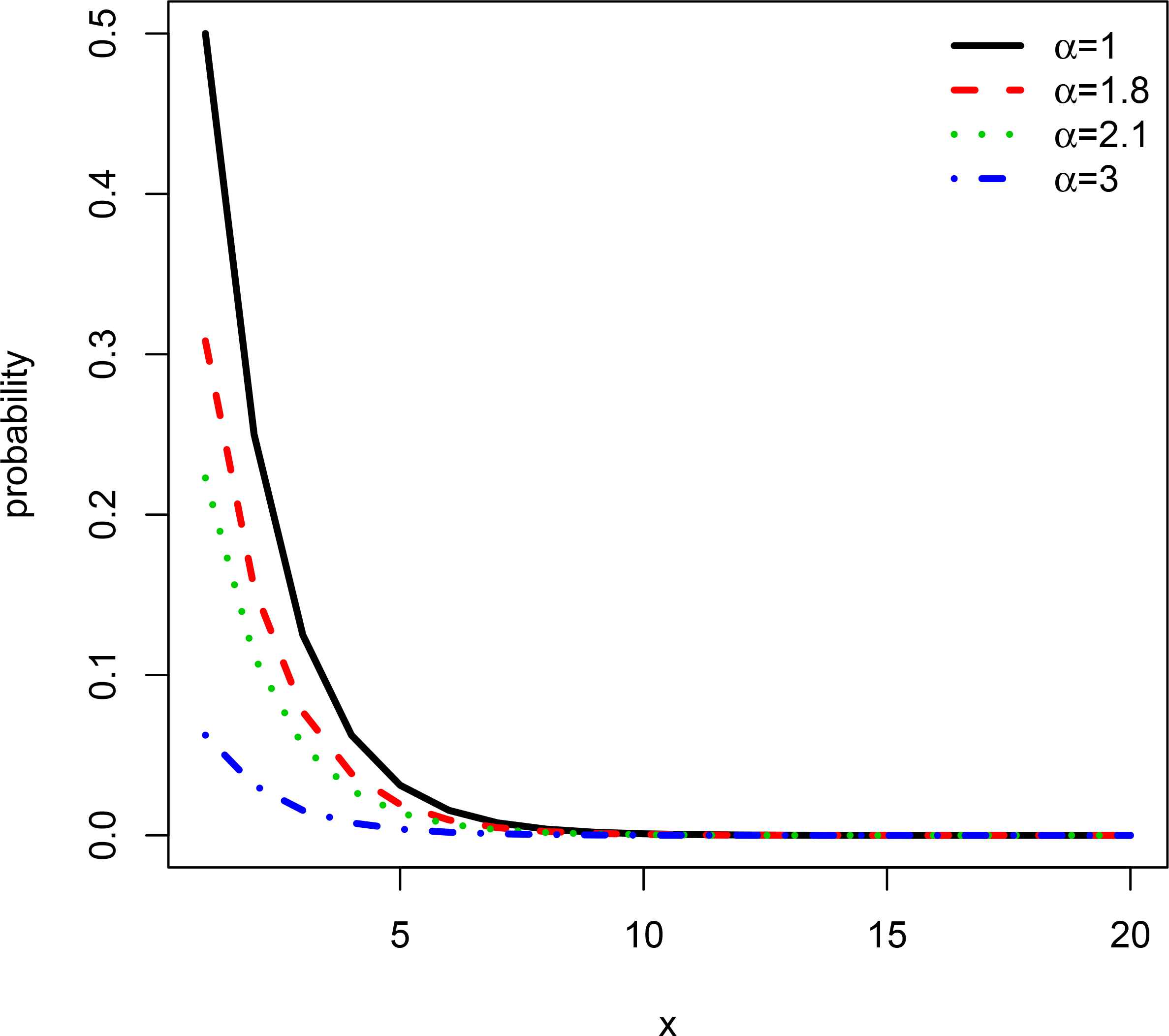
Probability mass functions (Γ∆) for various values of α and β = 0.5
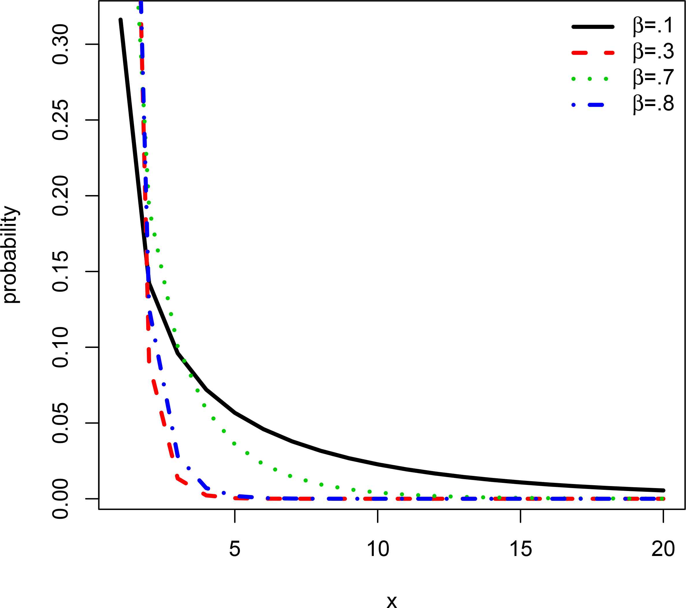
Probability mass functions (Γ∆) for various values of β and α = 0.5
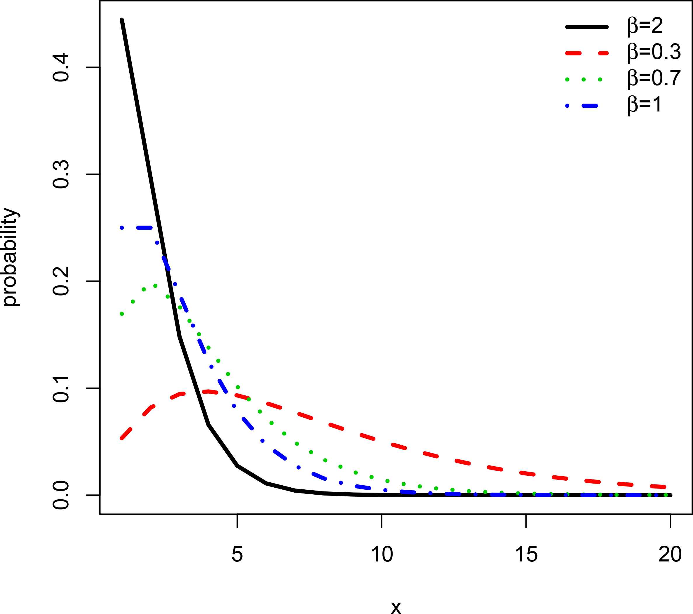
Probability mass functions (Γ∆) for various values of β and α = 2
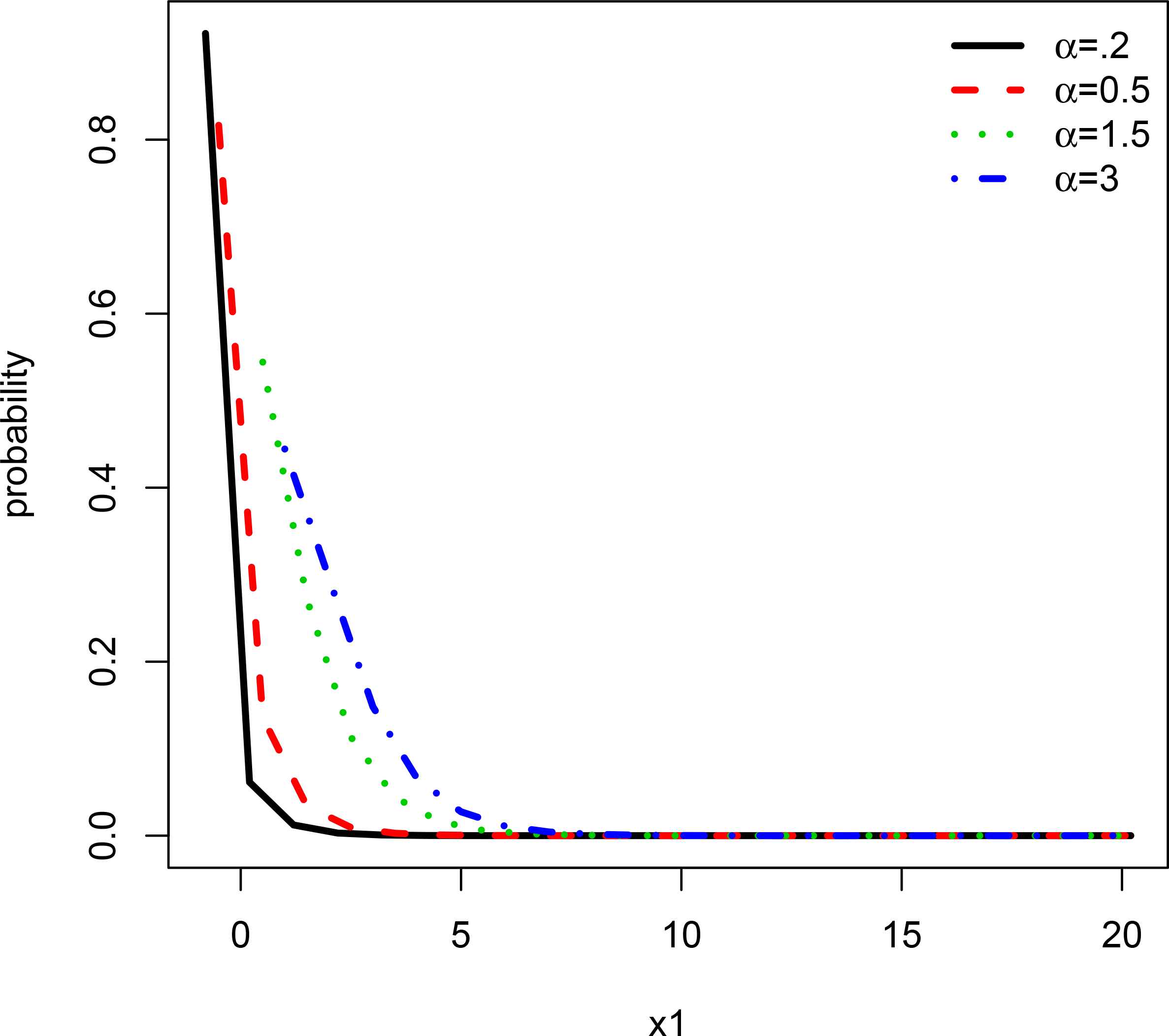
Probability mass functions (Γ∆) for various values of α and β = 2
References
Cite this article
TY  - JOUR
AU  - M. Ganji
AU  - F. Gharari
PY  - 2018
DA  - 2018/03/31
TI  - A New Method for Generating Discrete Analogues of Continuous Distributions
JO  - Journal of Statistical Theory and Applications
SP  - 39
EP  - 58
VL  - 17
IS  - 1
SN  - 2214-1766
UR  - https://doi.org/10.2991/jsta.2018.17.1.4
DO  - 10.2991/jsta.2018.17.1.4
ID  - Ganji2018
ER  -