Journal of Statistical Theory and Applications

Volume 17, Issue 1, March 2018, Pages 15 - 28

Results on Cumulative Measure of Inaccuracy in Record Values

Authors
Saeid Tahmasebi*, tahmasebi@pgu.ac.ir
Department of Statistics, Persian Gulf University, Bushehr, Iran
Ahmad Nezakatinezakati@shahroodut.ac.ir
Department of Statistics, Shahrood University of Technology, Iran
Safeih Daneshisdaneshi445@gmail.com
Department of Statistics, Shahrood University of Technology, Iran
*Corresponding
Corresponding Author
Saeid Tahmasebitahmasebi@pgu.ac.ir
Received 24 March 2016, Accepted 19 November 2017, Available Online 31 March 2018.
DOI
10.2991/jsta.2018.17.1.2How to use a DOI?
Keywords
Measure of inaccuracy; Cumulative inaccuracy; Record values
Abstract

In this paper, we propose cumulative measure of inaccuracy in lower record values and study characterization results in case of dynamic cumulative inaccuracy. We also discuss some properties of the proposed measures. Finally, we study a problem of estimating the cumulative measure of inaccuracy by means of the empirical cumulative inaccuracy in lower record values.

Copyright
Copyright © 2018, the Authors. Published by Atlantis Press.
Open Access
This is an open access article under the CC BY-NC license (http://creativecommons.org/licences/by-nc/4.0/).

1. Introduction

Let X and Y be two non-negative random variables with distribution functions F(x), G(x) and reliability functions F¯(x), G¯(x)), respectively. If f(x) is the actual probability density function(pdf) corresponding to the observations and g(x) is the density assigned by the experimenter, then the inaccuracy measure of X and Y is defined by Kerridge(1961) as

I(X,Y)=I(f,g)=0+f(x)logg(x)dx.
It has applications in statistical inference, estimation and coding theory. Analogous to the Kerridge measure of inaccuracy (1.1) , Thapliyal and Taneja (2015a) proposed a cumulative inaccuracy measure as
I(F,G)=0+F(x)logG(x)dx.
The mean inactivity time (MIT) function is of interest in many fields such as reliability, survival analysis, actuarial studies, etc. MIT of a random variable X is defined as
μ1(t)=E(tX|X<t).
Ghosh and Kundu (2017) obtained a connection between µ1(t) and I(F, G) as
I(F,G)=E(μ1(Y)F(Y)G(Y)).
Let X1, X2, ... be a sequence of iid random variables having an absolutely cdf F(x) and pdf f(x). An observation Xj is called a lower record value if its value is less than that of all previous observations. Thus, Xj is a lower record if Xj < Xi for every i < j. An analogous definition can be given for upper record values. Then the record times sequence Tn, n ≥ 1 is defined in the following manner: T1 = 1, with probability 1, and for n ≥ 2, Tn = min{j : j > Tn−1, Xj < XTn−1}. The lower record value sequence can be defined by Ln = XTn, n ≥ 1. Then the density function and cdf of Ln, which are denoted by fLn and FLn, respectively, are given by
fLn(x)=[logF(x)]n1(n1)!f(x),
FLn(x)=j=0n1[logF(x)]jj!F(x).
Record values are applied in problems such as industrial stress testing, meteorological analysis, hydrology, sporting and economics. In reliability theory, records values are used to study, for example, technical systems which are subject to shocks, e.g. peaks of voltages. For more details about records and their applications, one may refer to Arnold et al.(1992). Several authors have worked on measures of inaccuracy for ordered random variables. Thapliyal and Taneja (2013) proposed the measure of inaccuracy between the ith order statistic and the parent random variable. Thapliyal and Taneja (2015a) developed measures of dynamic cumulative residual and past inaccuracy. They studied characterization results of these dynamic measures under proportional hazard model and proportional reversed hazard model. Recently Thapliyal and Taneja (2015b) have introduced the measure of residual inaccuracy of order statistics and prove a characterization result for it. In this paper we propose cumulative past measure of inaccuracy and study their characterization results. The paper is organized as follows: In Section 2, we consider a measure of inaccuracy associated with FLn and F and obtain some results of its properties. In Section 3, we study dynamic version of inaccuracy associated with FLn and F. In Section 4, we propose empirical cumulative measure of inaccuracy in lower record values. Throughout the paper we assume that the terms increasing and decreasing are used in non-strict sense.

2. Cumulative measure of inaccuracy

The cumulative measure of inaccuracy between FLn (distribution function of nth lower record value Ln) and F is presented as

I(FLn,F)=0FLn(x)logF(x)dx=0F(x)j=0n1[logF(x)]jj!logF(x)dx=j=0n10[logF(x)]j+1j!logF(x)dx=j=0n1(j+1)0[logF(x)]j+1(j+1)!f(x)1λ˜(x)dx=j=0n1(j+1)ELj+2[1λ˜(X)],
where λ˜(x)=f(x)F(x) is the reversed hazard rate and Lj+2 is a random variable with density function fLj+2(x)=[logF(x)]j+1f(x)(j+1)!.

In the following, we present some examples and properties of I(FLn, F).

Example 2.1.

  1. i.

    If X has a inverse Weibull distribution with the cdf F(x)=exp((αx)β), x > 0. Then, we have

    I(FLn,F)=αβj=0n1Γ((j+1)β1β)j!.

    Figure 1 shows the function I(FLn, F) for α = β = 2. It is an increasing function of n.

  2. ii.

    If X is uniformly distributed in [0, θ]. Then, we obtain

    I(FLn,F)=θj=0n1(j+1)(12)j+1.

    From Figure 1 it is clear that I(FLn, F) for standard uniform distribution is increasing function of n and limn→∞ I(FLn, F) = 2θ.

  3. iii.

    If X is exponentially distributed with mean 1λ. Then, we obtain

    I(FLn,F)=1λj=0n1k=0(j+1)[1k+2]j+2.
    From Figure 1 it is clear that I(FLn, F) for exponential distribution with mean 12 is increasing function of n and limnI(FLn,F)=1.644λ.

Fig. 1.

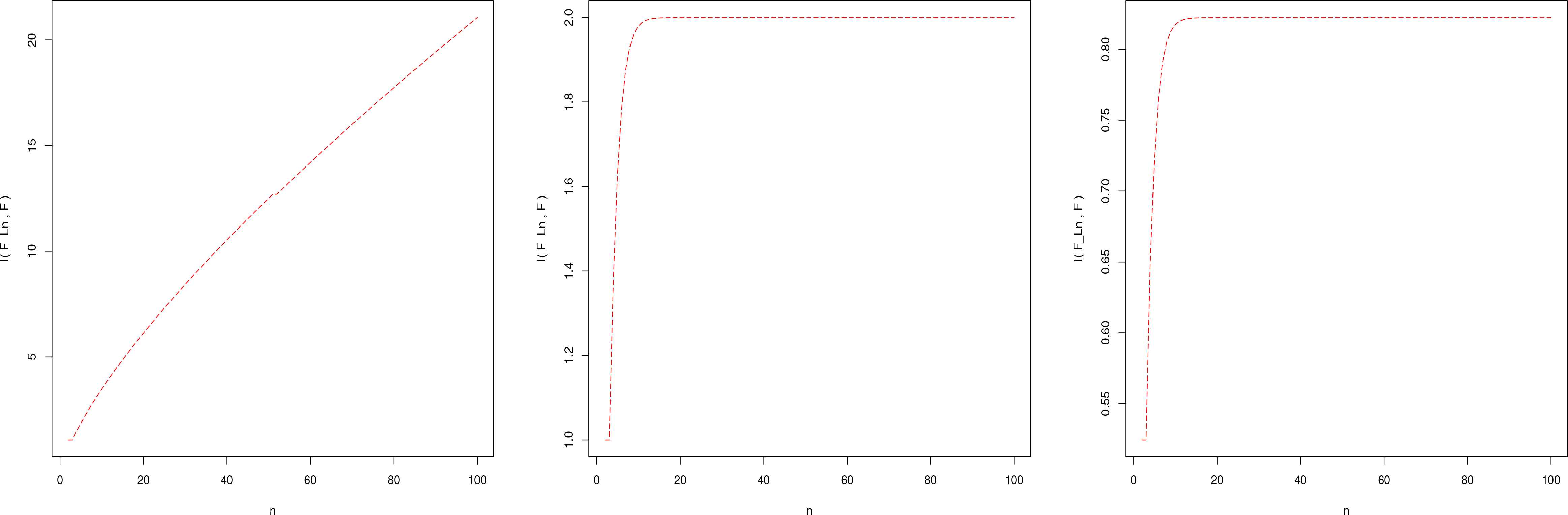
Plot of I(FLn, F) in inverse Weibull distribution for α = β = 2 (left), uniform distribution on (0, 1) (middle) and exponential distribution with λ = 2(right).

Proposition 2.1.

Suppose that X is a non-negative random variable with cdf F, then we have

I(FLn,F)=0j=0n1(j+1)[FLj+2(x)FLj+1(x)]dx.

Proof.

The proof follows from (1.4) and (2.1).

Proposition 2.2.

Let X be a non-negative random variable with cdf F, then we have

I(FLn,F)=j=0n11j!0λ˜(z)[0z[logF(x)]jF(x)dx]dz.

Proof.

By (2.1) and the relation logF(x)=xλ˜(z)dz, we have

I(FLn,F)=j=0n10[logF(x)]jj!F(x)dx=j=0n10[xλ˜(z)dz][logF(x)]jj!F(x)dx=j=0n11j!0λ˜(z)[0z[logF(x)]jF(x)dx]dz.
So, the proof is completed.

Proposition 2.3.

Let X be a non-negative random variable with cdf F, then an analytical expression for I(FLn, F) is given by

I(FLn,F)=j=0n10[logF(x)]j+1j!F(x)dx=j=0n1(j+1)𝒞j+1(X),
where
𝒞j+1(X)=0[logF(x)]j+1(j+1)!F(x)dx,
is a generalized cumulative entropy (see Kayal (2016)).

Proposition 2.4.

Let a, b > 0 for n = 1, 2, .... It holds that

I(FaLn+b,FaX+b)=aI(FLn,F).

Proof.

From (2.3) , we have

I(FaLn+b,FaX+b)=j=0n1(j+1)𝒞j+1(aX+b)=aj=0n1(j+1)𝒞j+1(X)=aI(FLn,F).

The proof is completed.

Proposition 2.5.

Let X be a absolutely continue non-negative random variable with I(FLn, F) < ∞, for all n ≥ 1. Then we have

I(FLn,F)=j=0n11j!E(h˜j+1(T)),
where h˜j+1(t)=t[logF(x)]j+1dx.

Proof.

By using (2.1) and Fubini’s theorem we obtain

I(FLn,F)=j=0n10[logF(x)]j+1j![0xf(t)dt]dx=j=0n10f(t)j![t[logF(x)]j+1dx]dt=j=0n11j!E[h˜j+1(T)].

Remark 2.1.

Let X be a symmetric random variable with respect to the finite mean µ = E(X), i.e. F(x + µ) = 1 − F(µ − x) for all x ∈ ℝ. Then

I(FLn,F)=I(F¯Rn,F¯),
where I(F¯Rn,F¯) is the cumulative residual measure of inaccuracy between F¯Rn (survival function of nth upper record value Rn) and F¯.

Kayal (2016) defined the MIT of lower record values as

μn(t)=E[tLn|Lnt]=0tFLn(x)dxFLn(t)=j=0n10tF(x)[logF(x)]jj!dxj=0n1F(t)[logF(x)]jj!.
Note that μ1(t)=0tF(x)dxF(t) is the MIT of the parent distribution. Now we consider a connection between µn(t) and I(FLn, F).

Proposition 2.6.

Let X be a non-negative random variable with cdf F, then we have

I(FLn,F)=j=0n1E[μn(Xj+1)].

Proof.

From (2.2) we have

I(FLn,F)=j=0n11j!0λ˜(z)[0z[logF(x)]jF(x)dx]dz=0λ˜(z)j=0n11j![0z[logF(x)]jF(x)dx]dz=0λ˜(z)μn(z)[j=0n11j![logF(z)]jF(z)]dz=0μn(z)[j=0n11j!f(z)[logF(z)]j]dz=j=0n10μn(z)fLj+1(z)=j=0n1E[μn(Xj+1)].
Hence, the desired result follows.

Proposition 2.7.

Suppose that X is a non-negative random variable with cdf F, then we have

I(FLn,F)=j=0n11j![i=0j1i!E[(logF(X))iμj+1(X)]i=0j11i!E[(logF(z))iμj(X)]].

Proof.

By using (1.4) and (2.2) we obtain

I(FLn,F)=j=0n11j!0λ˜(z)[0z[FLj+1(x)FLj(x)]dx]dz=j=0n11j!0λ˜(z)[μj+1(z)FLj+1(z)μj(z)FLj(z)]dz=j=0n11j!(i=0j1i!0f(z)[logF(z)]iμj+1(z)dzi=0j11i!0f(z)[logF(z)]iμj(z)dz)
This completes the proof.

Remark 2.2.

Let X be a non-negative random variable with cdf F and Xi+1 be the (i + 1) th lower record with pdf fLi+1(x). Then for n ≥ 1, we have

I(FLn,F)=j=0n1i=0j1j![E[μj+1(Xi+1)]E[μj(Xi+1)]].

Proof.

The proof follows from Proposition 2.7.

Remark 2.3.

In analogy with (2.1) , a measure of cumulative past inaccuracy associated with F and FLn is given by

I(F,FLn)=𝒞(X)E[Ulog(j=0n1(logU)jj!)f(F1(U))],
where 𝒞(X)=0F(x)logF(x)dx is the cumulative entropy(see Di Crescenzo and Longobardi (2009)).

In the sequel we obtain upper bound of I(F, FLn).

Proposition 2.8.

Let X be a non-negative random variable that take values in [0, a]. Then,

I(F,FLn)[aE(X)]|log(1E(Ln)a)|

Proof.

The proof follows from Proposition 1.9 of Ghosh and Kundu(2017) with the help of log-sum inequality.

In the next propositions we recall some lower bounds for I(FLn, F).

Proposition 2.9.

If X denotes an absolutely continue non-negative random variable with mean µ = EX < ∞. Then for n ≥ 1, we have

I(FLn,F)j=0n1h˜j+1(μ)j!,
where the function h˜j+1(.) is defined in Proposition 2.5.

Proof.

From (2.3) we have

I(FLn,F)=j=0n1(j+1)𝒞j+1(X)=j=0n1E(h˜j+1(X))j!.
Since h˜j+1(X) is a convex function, applying Jensen’s inequality we obtain
I(FLn,F)j=0n1h˜j+1(μ)j!.

Proposition 2.10.

Let X be a non-negative random variable with cdf F, then we have

I(FLn,F)=j=0n1(j+1)𝒞j+1(X)j=0n1[𝒞(X)]j+1j!,
where 𝒞ℰ(X) is given in Remark 2.3(For more details see Di Crescenzo and Longobardi (2009)).

Proof.

Since (F(x))nF(x), for all n = 1, 2, ..., we have

I(FLn,F)=j=0n10(logF(x))j+1j!F(x)dxj=0n10(logF(x))j+1j!(F(x))j+1=j=0n10[(logF(x))F(x)]j+1j!dxj=0n11j![0(logF(x))F(x)dx]j+1,
which immediately follows (2.9) .

Remark 2.4.

Let X be a non-negative random variable with cdf F, then for n = 1, 2, ... we have

I(FLn,F)j=0n11j![0F(x)F¯(x)dx]j+1.

Proof.

By using Proposition 4.3 of Dicresenzo and Longobardi (2009) a lower bound for 𝒞ℰ(X) is

𝒞(X)0F(x)F¯(x)dx.
Now, Proposition 2.10 completes the proof.

Proposition 2.11.

For a non-negative random variable and n = 1, 2, ..., we have

I(FLn,F)j=0n11j![μ.gini(X)]j+1,
where µ = E(X) and gini[.] is the Gini index, a celebrated measure of income inequality denoted by(see Wang 1998)
gini[X]=10[F¯(x)]2dxE(X).

Proof.

From Proposition 5.1 of Wang (1998), we have

0F(x)F¯(x)dx=12E(|XY|)=E(X).gini[X],
where X and Y are independent and have the same distributions. Hence, Eq (2.10) completes the proof.

Corollary 2.1.

Let X be a non-negative random variable with survival function F¯(x), then we have

I(FLn,F)j=0n11j!cj+1e(j+1)H(X),
where c=exp(01log(x|logx|)dx)=0.2065 and H(X)=0f(x)logf(x)dx is the Shannon entropy of X.

Proof.

The proof follows by recalling (2.9) and Proposition 4.2 of Di Crescenzo and Longobardi (2009).

Now we can prove an important property of inaccuracy measure using some properties of stochastic ordering. For that we present the following definitions:

  1. 1.

    The random variable X is said to be smaller than Y according to stochastically ordering (denoted by X ≤st Y) if P(X ≥ x) ≤ P(Y ≥ x) for all x. It is known that X ≤st YE(ϕ(X)) ≤ E(ϕ(Y)) for all increasing functions ϕ such that the expectations exist.

  2. 2.

    The random variable X is said to be smaller than Y in likelihood ratio ordering(denoted by X ≤lr Y) if g(x)f(x) is increasing in x.

  3. 3.

    A random variable X is said to be smaller than a random variable Y in the decreasing convex order, denoted by X ≤dcx Y, if E(ϕ(X)) ≤ E(ϕ(Y)) for all decreasing convex functions ϕ such that the expectations exist.

  4. 4.

    A non-negative random variable X is said to have decreasing reversed hazard rate DRHR if λ˜F(x)=f(x)F(x) is decreasing in x.

Theorem 2.1.

Suppose that the non-negative random variable X is DRHR, then

I(FLn+1,F)I(FLn,F)i=1n+1ELi[1λ˜(X)].

Proof.

Let fLn(x) be the pdf of n-th lower record value XLn. Then, the ratio fLn(x)fLn+1(x)=nlogF(x) is increasing in x. Therefore, Xn+1lr Xn, and this implies that Xn+1st Xn, i.e. F¯n+1(x)F¯n(x) (For more details see Shaked and Shanthikumar( 2007,Chapter 1)). This is equivalent (see Shaked and Shanthikumar (2007,p.4)) to have

E(φ(Xn+1))E(φ(Xn)),
for all increasing functions ϕ such that these expectations exist. Thus, if X is DRHR and λ˜(x) is its reversed hazard rate, then 1λ˜(x) is increasing in x. As a consequence, from (2.1) we have
I(FLn+1,F)=j=0n(j+1)ELj+2[1λ˜(X)]j=0n(j+1)ELj+1[1λ˜(X)]=i=1n1(i+2)ELj+2[1λ˜(X)]=i=0n1(i+2)ELi+2[1λ˜(X)]+EL1[1λ˜(X)]=I(FLn,F)+i=1n+1ELi[1λ˜(X)].
Thus the proof is completed.

Theorem 2.2.

Let X and Y be two non-negative random variables such that X ≤dcx Y, then we have

I(FLn,F)I(GLn,G).

Proof.

Since h˜j+1(x) is a decreasing convex function in x. Then the proof immediately follows from (2.7) .

Proposition 2.12.

Let X be a non-negative random variable with absolutely continuous cumulative distribution function F(x). Then for n = 1, 2, ... we have

I(FLn,F)j=0n1i=0j+1(1)i(j+1)i!(j+1i)!0[F(x)]i+1dx.

Proof.

Since −logF(x) ≥ 1 − F(x), the proof follows by recalling (2.1) .

Proposition 2.13.

Let X be a non-negative random variable with absolutely continuous cumulative distribution function F(x). Then for n = 1, 2, ... we have

I(FLn,F)j=0n11j!0[logF(x)]j+1dx.

Assume that X˜θ denotes a nonnegative absolutely continuous random variable with the distribution function Hθ(x) = [F(x)]θ, x ≥ 0. We now obtain the cumulative measure of inaccuracy between HLn and H as follows:

I(HLn,H)=0+HLn(x)log(H(x))dx=j=0n1θj+10+[logF(x)]j+1j![F(x)]θdx.

Proposition 2.14.

If θ ≥ (≤)1, then for any n = 1, 2, ... we have

I(HLn,H)=j=0n1(j+1)𝒞j+1(X˜θ)()j=0n1θj+1(j+1)𝒞j+1(X).

Proof.

Suppose that θ ≥ ()1, then it is clear [F(x)]θ ()F(x), and hence we have

I(HLn,H)=j=0n1(j+1)𝒞j+1(X˜θ)()j=0n1θj+1(j+1)𝒞j+1(X).

3. Dynamic cumulative measure of inaccuracy

In the reliability theory dynamical measures are useful to describe the information content carried by random lifetimes as age varies. In this section, we study dynamic version of I(FLn, F). If a system that begins to work at time 0 is observed only at deterministic inspection times, and is found to be down at time t, then we consider a dynamic cumulative measure of inaccuracy as

I(FLn,F;t)=0tFLn(x)FLn(t)log(F(x)F(t))dx=logF(t)μn(t)0tFLn(x)FLn(t)log(F(x))dx=logF(t)μn(t)+1FLn(t)j=0n10t[logF(x)]j+1j!F(x)dx.

Note that limtI(FLn,F;t)=(FLn,F). Since logF(t) 0 for t ≥ 0, we have

I(FLn,F;t)1FLn(t)j=0n10t[logF(x)]j+1j!F(x)dx1FLn(t)j=0n10+[logF(x)]j+1j!F(x)dx=I(FLn,F)FLn(t).
In the following theorem, we prove that I(FLn, F;t) uniquely determine the distribution function.

Theorem 3.1.

Let X be a nonnegative continuous random variable with distribution function F(.). Let the dynamic cumulative inaccuracy of the nth lower record value denoted by I(FLn, F;t) < ∞, t ≥ 0. Then I(FLn, F;t) characterizes the distribution function.

Proof.

From (3.1) we have

I(FLn,F;t)=logF(t)μn(t)+1FLn(t)j=0n10t[logF(x)]j+1j!F(x)dx.
Differentiating both side of (3.2) with respect to t we obtain:
ddt[I(FLn,F;t)]=λ˜F(t)μn(t)λ˜FLn(t)I(FLn,F;t)=λ˜F(t)μn(t)c(t)λ˜F(t)I(FLn,F;t)=λ˜F(t)[μn(t)c(t)I(FRn,F;t)].
Taking derivative with respect to t again we get
λ˜´=(λ˜F(t))2[c´(t)I(FLn,F;t)+c(t)I´(FLn,F;t)1+c(t)λ˜F(t)μn(t)]I´(FLn,F;t).
Suppose that there are two functions F and F * such that
I(FLn,F;t)=I(FLn*,F*;t)=z(t).

Then for all t, from (3.3) we get

λ˜´F(t)=ϕ(t,λ˜´F(t)),λ˜F(t)=ϕ(t,λ˜F*(t)),
where
ϕ(t,y)=y2[ç(t)z(t)c´(t)z´(t)1+c(t)yw(t)]z´(t),
and w(t) = µn(t). By using Theorem (2.1) and Lemma (2.2) of Gupta and Kirmani(2008), we have λ˜F(t)=λ˜F*(t), for all t. Since the reversed hazard rate function characterizes the distribution function uniquely, we complete the proof.

4. Empirical cumulative measure of inaccuracy

In this section we study the problem of estimating the cumulative measure of inaccuracy by means of the empirical cumulative inaccuracy in lower record values. Let X1, X2, ..., Xm be a random sample of size m from an absolutely continuous cumulative distribution function F(x). Then according to (2.3), the empirical cumulative measure of inaccuracy is defined as

I^(FLn,F)=j=0n10[logF^m(x)]j+1j!F^m(x)dx=j=0n1(j+1)𝒞j+1(F^m),
where
F^m(x)=1mi=1mI(Xix),x.
is the empirical distribution of the sample and I is the indicator function. If we denote X(1) ≤ X(2) ≤ ... ≤ X(m) as the order statistics of the sample, then (4.1) can be written as
I^(FLn,F)=j=0n1k=1m1X(k)X(k+1)[logF^m(x)]j+1j!F^m(x)dx.
Moreover,
F^m(x)={0,x<X(1),km,X(k)xX(k+1),k=1,2,,j1,x>X(k+1).
Hence, (4.2) can be written as
I^(FLn,F)=j=0n1k=1m11j!Uk+1km(lnkm)j+1,
where Uk+1 = X(k+1) − X(k), k = 1, 2, ..., m − 1 are the sample spacings.

Example 4.1.

Let X1, X2, ..., Xm be a random sample drawn from exponential distribution with mean 1λ. Then the sample spacings Uk+1 are independent and exponentially distributed with mean ë(m − k) (for more details see Pyke (1965)). Now from (4.3) we obtain

E[I^(FLn,F)]=1λj=0n1k=1m11j!(mk)(km)(lnkm)j+1,
and
Var[I^(FLn,F)]=1λ2j=0n1k=1m11(j!)2(mk)2(km)2(lnkm)2(j+1).
We have computed the values of E[Î(FLn, F)] and Var[Î(FLn, F)] for sample sizes m = 10, 15, 20, ë = 0.5, 1, 2 and n = 2, 3, 4, 5 in Table 1. We can easily see that E[Î(FLn, F)] is increasing in m. Also, we consider that Var[Î(FLn, F)] is decreasing in m.

E[Î(FLn, F)]

α 0.5 1 2 0.5 1 2 0.5 1 2 0.5 1 2

m n = 2 n = 3 n = 4 n = 5
10 1.96 0.980 0.490 2.395 1.197 0.598 2.614 1.307 0.653 2.711 1.355 0.677
15 2.011 1.005 0.502 2.471 1.235 0.617 2.716 1.358 0.679 2.834 1.417 0.708
20 2.035 1.017 0.508 2.506 1.253 0.626 2.765 1.382 0.691 2.896 1.448 0.724
Var[Î(FLn, F)]

α 0.5 1 2 0.5 1 2 0.5 1 2 0.5 1 2

m n = 2 n = 3 n = 4 n = 5
10 0.252 0.063 0.015 0.291 0.072 0.018 0.306 0.076 0.0191 0.310 0.077 0.0194
15 0.173 0.043 0.010 0.201 0.050 0.012 0.214 0.053 0.013 0.219 0.054 0.013
20 0.131 0.032 0.008 0.153 0.038 0.009 0.164 0.041 0.010 0.168 0.042 0.0105
Table 1.

Numerical values of E[Î(FLn, F)] and Var[Î(FLn, F)] for exponential distribution.

E[Î(FLn, F)] var[Î(FLn, F)]

m n=2 n=3 n=4 n=5 n=2 n=3 n=4 n=5
10 0.437 0.581 0.660 0.697 0.014 0.019 0.021 0.022
15 0.459 0.619 0.713 0.760 0.010 0.014 0.016 0.017
20 0.470 0.637 0.739 0.794 0.007 0.011 0.013 0.014
Table 2.

Numerical values of E[Î(FLn, F)] and Var[Î(FLn, F)] for uniform distribution.

Example 4.2.

Let X1, X2, ..., Xm be a random sample from a population uniformly distributed in (0, 1). Then the sample spacings Uk+1 are independent of beta distribution with parameters 1 and m (for more details see Pyke (1965)). Now from (4.3) we obtain

E[I^(FLn,F)]=j=0n1k=1m11j!(m+1)(km)(lnkm)j+1,
and
Var[I^(FLn,F)]=j=0n1k=1m11(j!)2(m)(m+2)(km)2(lnkm)2(j+1).
We have computed the values of E[Î(FLn, F)] and Var[Î(FLn, F)] for sample sizes m = 10, 15, 20 and n = 2, 3, 4, 5. We can easily see that E[Î(FLn, F)] is increasing in m and n. Also, we consider that limmVar[I^(FLn,F)]=0.

Conclusions

In this paper, we discussed on concept of inaccuracy between FLn and F. We proposed a dynamic version of cumulative inaccuracy and studied characterization results of it. It is also proved that I(FLn, F;t) can uniquely determine the parent distribution F. Moreover, we studied some new basic properties of I(FLn, F) and I(FLn, F;t) such as the stochastic order properties. We also constructed bounds for characterization results of I(FLn, F). Finally, we estimated the cumulative measure of inaccuracy by means of the empirical cumulative inaccuracy in lower record values. These concepts can be applied in measuring the inaccuracy contained in the associated past lifetime.

References

[3.]A Ghosh and C Kundu, Bivariate extension of (dynamic) cumulative residual and past inaccuracy measures, 2017. Stat Papers.
Journal
Journal of Statistical Theory and Applications
Volume-Issue
17 - 1
Pages
15 - 28
Publication Date
2018/03/31
ISSN (Online)
2214-1766
ISSN (Print)
1538-7887
DOI
10.2991/jsta.2018.17.1.2How to use a DOI?
Copyright
Copyright © 2018, the Authors. Published by Atlantis Press.
Open Access
This is an open access article under the CC BY-NC license (http://creativecommons.org/licences/by-nc/4.0/).

Cite this article

TY  - JOUR
AU  - Saeid Tahmasebi
AU  - Ahmad Nezakati
AU  - Safeih Daneshi
PY  - 2018
DA  - 2018/03/31
TI  - Results on Cumulative Measure of Inaccuracy in Record Values
JO  - Journal of Statistical Theory and Applications
SP  - 15
EP  - 28
VL  - 17
IS  - 1
SN  - 2214-1766
UR  - https://doi.org/10.2991/jsta.2018.17.1.2
DO  - 10.2991/jsta.2018.17.1.2
ID  - Tahmasebi2018
ER  -