
Inferences for the Type-II Exponentiated Log-Logistic Distribution Based on Order Statistics with Application
 , Maneesh Kumar1, Sanku Dey2
- DOI
- 10.2991/jsta.d.200825.002How to use a DOI?
- Keywords
- Type-II exponentiated log-logistic distribution; Moments; Order statistics; Best linear unbiased estimators
- Abstract
In this paper, we first derive the exact explicit expressions for the single and product moments of order statistics from the type-II exponentiated log-logistic distribution, and then use these results to compute the means, variances, skewness and kurtosis of rth order statistics. Besides, best linear unbiased estimators (BLUEs) for the location and scale parameters for the type-II exponentiated log-logistic distribution with known shape parameters are studied. Finally, the results are illustrated with a real data set.
- Copyright
- © 2020 The Authors. Published by Atlantis Press B.V.
- Open Access
- This is an open access article distributed under the CC BY-NC 4.0 license (http://creativecommons.org/licenses/by-nc/4.0/).
1. INTRODUCTION
Rao et al. (2012) suggested a generalization of the log-logistic distribution called type-II exponentiated log-logistic (TIIELL) distribution with probability density function (pdf)
The cumulative distribution function (cdf) and quantile function are, respectively given by
Therefore,
To the best of our knowledge, the work on type-II generalized log-logistic model is scanty in literature. The few works available in literature on this distribution which includes: Rao et al. [2,3] developed the reliability and an economic reliability test plans for this distribution. Kumar [4] studied exact moments of generalized order statistics from TIIELL distribution. Recently, Rao et al. [5] studied Bootstrap confidence intervals (CIs) of the process capability index,
Order statistics and functions of these statistics occupy a place of great significance in diverse field of studies involving theoretical and practical problems such as characterization of probability distributions, entropy estimation, analysis of censored samples, reliability analysis and quality control (see Arnold et al. [6] and David and Nagaraja [7]). The moments of order statistics have applicability in areas such as quality control, reliability, etc. For example, it is seen that when the duration of the failed items is high, the reliability of an item is also high, which in turn makes the product too costly, both in terms of time and money. In such a situation the one may not know enough about the item in a short period of time and hence would require few early failures data for predicting the failure of future items. Thus moments of order statistics is useful in making these kinds of prediction in such situations.
In recent past several authors have tabulated the moments of order statistics quite extensively for several distributions and also obtained maximum likelihood estimates (MLEs) and best linear unbiased estimators (BLUEs) for the scale and location parameters of the distributions based on complete and type-II censored samples. Further, they developed point prediction and goodness-of-fit tests. In this regard, readers may refer to the works of Balakrishnan and Cohan [8], Balakrishnan and Sultan [8], Sultan and Balakrishnan [9,10], Genç [11], Jabeen et al. [12], Mir Mostafaee [13], Balakrishnan et al. [14], Sultan and AL-Thubyani [15], Kumar et al. [16], Kumar and Dey [17,18], Ahsanullah and Alzaatreh [19], Kumar and Goyal [20,21], Kumar et al. [22] and many others.
In this paper, we derive the exact expressions for the single and product moments of order statistics from TIIELLD in Sections 2 and 3. In Section 4, we obtain BLUEs for
2. SOME RELATIONS FOR THE MOMENTS OF ORDER STATISTICS
Let
The
Theorem 1.
For the TIIELL distribution given in equation (1) and for
Proof.
From equation (7), we have
Theorem 2.
For the TIIELL distribution given in equation (1) and for
Proof.
The proof is straightforward and omitted for brevity.
Note that from equation (9), the first and second moments of
Some special cases from equation (9) are
For
If
which agrees with equation (4).If
If
If
which agree with equation (5) for
It is interesting to note that the equation (9) can be used easily to derive several recurrence relations for the moments of order statistics. Some of these recurrence relations already exist in the literature. Below, we provide some of these recurrence relations.
I. From equation (9), we can write
Let us define
Therefore, we can write
3. PRODUCT MOMENTS OF ORDER STATISTICS
Let
Therefore, the product moments of
Theorem 3.
For the TIIELL distribution given in (1) and for
Proof
From equation (12), we have
4. ESTIMATION OF PARAMETERS
4.1. Estimation of the Location and Scale Parameters
In this section, we study parameter estimation for the TIIELL distribution based on order statistics. Let
Let
| m | s | |||||||||||
|---|---|---|---|---|---|---|---|---|---|---|---|---|
| 2 | 7 | 0 | 0.013963 | 0.101597 | 0.558978 | 0.263992 | 0.051795 | 0.009676 | −5.27E-07 | |||
| 1 | −0.34963 | 0.833878 | 0.401217 | 0.108408 | 0.006114 | 1.22E-05 | ||||||
| 2 | −0.11492 | 0.812707 | 0.290103 | 0.012084 | 2.69E-05 | |||||||
| 10 | 0 | 0.026562 | 0.067891 | 0.131564 | 0.228105 | 0.328165 | 0.132287 | 0.060663 | 0.023448 | 0.001311 | 3.53E-06 | |
| 1 | 0.039625 | 0.100778 | 0.188777 | 0.284606 | 0.265189 | 0.082232 | 0.036252 | 0.002535 | 4.15E-06 | |||
| 2 | 0.04799 | 0.127099 | 0.250121 | 0.374234 | 0.143044 | 0.053643 | 0.003868 | 1.68E-06 | ||||
| 3 | 0.029534 | 0.131456 | 0.511993 | 0.235 | 0.087684 | 0.00432 | 1.37E-05 | |||||
| 4 | −0.25036 | 0.761078 | 0.334894 | 0.145439 | 0.008938 | 9.13E-06 | ||||||
| 3 | 7 | 0 | −0.46467 | −0.74389 | 1.449078 | 0.545318 | 0.204818 | 0.009332 | 1.17E-05 | |||
| 1 | −0.29246 | −0.60828 | 1.444277 | 0.453126 | 0.003324 | 1.28E-05 | ||||||
| 2 | −1.58802 | 1.838166 | 0.728422 | 0.021388 | 4.29E-05 | |||||||
| 10 | 0 | −0.01692 | −0.03763 | −0.06087 | −0.04818 | 0.118261 | 0.764299 | 0.199978 | 0.078079 | 0.002988 | 1.05E-06 | |
| 1 | 0.002353 | 0.007739 | 0.019326 | 0.051598 | 0.170786 | 0.611624 | 0.131185 | 0.005383 | 5.88E-06 | |||
| 2 | −0.01192 | −0.03172 | −0.03954 | 0.060255 | 0.846969 | 0.166772 | 0.009176 | 7.58E-06 | ||||
| 3 | −0.06968 | −0.16761 | −0.15093 | 1.136136 | 0.240728 | 0.011335 | 2.05E-05 | |||||
| 4 | −0.29882 | −0.61856 | 1.540259 | 0.349781 | 0.027336 | 8.17E-06 |
Coefficient of the best linear unbiased estimators (BLUEs) of the
| m | s | |||||||||||
|---|---|---|---|---|---|---|---|---|---|---|---|---|
| 2 | 7 | 0 | −1.42624 | −2.69332 | 2.763219 | 1.092811 | 0.224505 | 0.039025 | −3.63E-06 | |||
| 1 | −5.05483 | 3.111726 | 1.515761 | 0.403758 | 0.023545 | 4.36E-05 | ||||||
| 2 | −4.45187 | 3.226687 | 1.177263 | 0.047808 | 0.000117 | |||||||
| 10 | 0 | −0.40703 | −0.92138 | −1.2938 | −0.64137 | 2.3615 | 0.5141 | 0.274523 | 0.107245 | 0.006194 | 1.47E-05 | |
| 1 | −0.28225 | −0.6877 | −1.08679 | −0.841 | 2.287784 | 0.409765 | 0.185349 | 0.014828 | 1.58E-05 | |||
| 2 | −0.56606 | −1.313 | −1.47408 | 2.431089 | 0.650346 | 0.253884 | 0.017819 | 7.43E-06 | ||||
| 3 | −1.34466 | −2.59115 | 2.584963 | 0.96291 | 0.369273 | 0.018615 | 5.26E-05 | |||||
| 4 | −4.68322 | 2.837779 | 1.270177 | 0.540726 | 0.034506 | 3.06E-05 | ||||||
| 3 | 7 | 0 | −2.17816 | −3.85459 | 4.049251 | 1.422057 | 0.537002 | 0.024409 | 3.09E-05 | |||
| 1 | −1.65382 | −3.79265 | 4.181823 | 1.255093 | 0.009517 | 3.47E-05 | ||||||
| 2 | −6.66135 | 4.733542 | 1.872912 | 0.054788 | 0.000108 | |||||||
| 10 | 0 | −0.21816 | −0.51608 | −0.92486 | −1.24654 | −0.76193 | 2.846231 | 0.570023 | 0.242188 | 0.009133 | 2.23E-06 | |
| 1 | −0.12748 | −0.32472 | −0.62717 | −1.01443 | −0.95517 | 2.569284 | 0.460068 | 0.019596 | 1.77E-05 | |||
| 2 | −0.25649 | −0.69056 | −1.2704 | −1.44404 | 3.097968 | 0.533783 | 0.029706 | 2.53E-05 | ||||
| 3 | −0.6069 | −1.57047 | −2.26163 | 3.697287 | 0.70758 | 0.03408 | 5.81E-05 | |||||
| 4 | −1.6753 | −3.83228 | 4.469613 | 0.962392 | 0.075552 | 2.27E-05 |
Coefficient of the best linear unbiased estimators (BLUEs) of the
5. APPROXIMATE INFERENCE
Here, we derive the
To derive the CIs of the location and scale parameters based on the pivotal quantities in equation (22), the moments presented in Section 2, are used.
Hence,
To obtain the coefficients of skewness and kurtosis of linear functions of order statistics, single moments
Table 3 displays the values of the mean, variance, coefficients of skewness and kurtosis
| n | c | ||||
|---|---|---|---|---|---|
| 2 | 7 | 0 | 0.074821 | 0.970035 | 0.253528 |
| 1 | 0.093972 | 1.102865 | 0.310651 | ||
| 2 | 0.125613 | 1.597531 | 0.426752 | ||
| 10 | 0 | 0.044879 | 0.616469 | 0.152306 | |
| 1 | 0.052941 | 0.848929 | 0.185043 | ||
| 2 | 0.060478 | 0.878651 | 0.209287 | ||
| 3 | 0.073563 | 0.955970 | 0.248770 | ||
| 4 | 0.087637 | 1.020583 | 0.287920 | ||
| 3 | 7 | 0 | 0.153237 | 0.952101 | 0.377268 |
| 1 | 0.214149 | 1.459957 | 0.549955 | ||
| 2 | 0.248820 | 1.525382 | 0.610006 | ||
| 10 | 0 | 0.106367 | 0.810697 | 0.284275 | |
| 1 | 0.132891 | 1.206524 | 0.379329 | ||
| 2 | 0.150195 | 1.238222 | 0.414675 | ||
| 3 | 0.182625 | 1.375398 | 0.488490 | ||
| 4 | 0.211345 | 1.424032 | 0.539068 |
Variances and covariance of the best linear unbiased estimators (BLUEs) when
The performance of the developed inference can be shown from the simulated average width of CIs in Table 10. We observe that the Edgeworth approximations of the distributions of
| n | c | 1% | 2.50% | 5% | 10% | 90% | 95% | 97.50% | 99% | |
|---|---|---|---|---|---|---|---|---|---|---|
| 2 | 7 | 0 | −0.7784 | −0.76196 | −0.73504 | −0.68271 | 1.083601 | 1.925702 | 1.854568 | 4.255494 |
| −1.03231* | −0.97438* | −0.90792* | −0.81937* | 1.083648* | 1.76806* | 2.560536* | 3.7586* | |||
| 1 | −2.27628 | −2.32369 | −0.67909 | −0.62752 | 0.20892 | 1.889575 | 1.822893 | 4.241948 | ||
| −1.4765* | −1.41945* | −1.35722* | −1.26558* | 0.682143* | 1.351194* | 2.104918* | 3.327379* | |||
| 2 | −2.34755 | −2.41664 | −2.56902 | −2.86364 | 0.324397 | 0.432937 | 1.791339 | 3.749634 | ||
| −2.0666* | −2.01487* | −1.95338* | −1.8637* | 0.126588* | 0.818807* | 1.556711* | 2.749675* | |||
| 10 | 0 | −0.63703 | −0.62091 | −0.59465 | −0.54415 | 1.968333 | 1.825218 | 3.499767 | 4.188481 | |
| −1.19869* | −1.11596* | −1.03013* | −0.90966* | 1.176293* | 1.81677* | 2.499808* | 3.605541* | |||
| 1 | −2.5634 | −1.08063 | −1.02533 | −0.92635 | 0.773829 | 1.106087 | 1.429446 | 3.896156 | ||
| −1.68973* | −1.60117* | −1.51202* | −1.38262* | 0.766383* | 1.428123* | 2.120552* | 3.137602* | |||
| 2 | −2.51757 | −2.77431 | −2.97307 | −2.89647 | 0.704014 | 0.993738 | 1.354706 | 3.585678 | ||
| −2.19815* | −2.10884* | −2.02115* | −1.89652* | 0.271168* | 0.924273* | 1.627683* | 2.585719* | |||
| 3 | −2.53477 | −3.16427 | −2.9827 | −2.98269 | 0.732411 | 1.042713 | 1.382714 | 1.382703 | ||
| −2.72401* | −2.63791* | −2.55189* | −2.42756* | −0.25733* | 0.390673* | 1.068124* | 2.10397* | |||
| 4 | −3.83866 | −3.30443 | −2.96218 | −2.96219 | 0.181199 | 0.835414 | 1.163553 | 1.314588 | ||
| −3.25567* | −3.17872* | −3.09859* | −2.98289* | −0.81876* | −0.16451* | 0.504467* | 1.485206* | |||
| 3 | 7 | 0 | −0.38025 | −0.37311 | −0.36123 | −0.33769 | 1.936298 | 1.888275 | 1.865233 | 4.491297 |
| −0.9566* | −0.90678* | −0.8515* | −0.77025* | 1.032663* | 1.716643* | 2.505057* | 3.743581* | |||
| 1 | −2.28575 | −2.32319 | −0.66079 | −0.61545 | 0.161453 | 1.927139 | 1.87266 | 4.263209 | ||
| −1.45259* | −1.40138* | −1.34743* | −1.268* | 0.586968* | 1.278905* | 2.080461* | 3.263277* | |||
| 2 | −2.30645 | −2.35543 | −2.45118 | −2.81325 | 0.226085 | 0.306988 | 1.837418 | 3.764807 | ||
| −1.991* | −1.94309* | −1.89224* | −1.81329* | 0.111492* | 0.792065* | 1.60848* | 2.764848* | |||
| 10 | 0 | −0.83021 | −0.81163 | −0.78146 | −0.72326 | 1.296581 | 1.916373 | 1.828839 | 4.202645 | |
| −1.0873* | −1.0183* | −0.94733* | −0.84676* | 1.096046* | 1.772315* | 2.542991* | 3.727137* | |||
| 1 | −2.18033 | −2.21922 | −2.29146 | −2.39668 | 0.156439 | 1.849359 | 1.797111 | 4.137826 | ||
| −1.65246* | −1.57954* | −1.5031* | −1.39675* | 0.607943* | 1.262664* | 2.027025* | 3.137897* | |||
| 2 | −2.41444 | −2.52619 | −2.92543 | −2.92543 | 0.480104 | 0.644207 | 1.703217 | 3.567014 | ||
| −2.28619* | −2.21093* | −2.12713* | −2.01619* | 0.051319* | 0.72511* | 1.48204* | 2.567054* | |||
| 3 | −2.44641 | −2.58122 | −2.94305 | −2.94304 | 0.424358 | 0.740532 | 0.873089 | 1.518757 | ||
| −2.94442* | −2.86884* | −2.78695* | −2.67421* | −0.57559* | 0.095727* | 0.809759* | 1.841936* | |||
| 4 | −3.94473 | −3.48833 | −2.95145 | −2.95145 | −0.14498 | 0.510946 | 0.891869 | 1.527782 | ||
| −3.48544* | −3.41859* | −3.34497* | −3.23734* | −1.14494* | −0.48899* | 0.243865* | 1.30883* |
Edgeworth approximate and the simulated (*) values of the distribution of
| n | c | 1% | 2.50% | 5% | 10% | 90% | 95% | 97.50% | 99% | |
|---|---|---|---|---|---|---|---|---|---|---|
| 2 | 7 | 0 | −0.68625 | −0.67387 | −0.65342 | −0.613 | 1.120145 | 1.963351 | 1.917835 | 4.386462 |
| −0.89515* | −0.85571* | −0.81026* | −0.74149* | 1.01628* | 1.700985* | 2.516495* | 3.864885* | |||
| 1 | −2.23387 | −2.26766 | −0.5896 | −0.54756 | 0.133227 | 1.900113 | 1.852216 | 4.326887 | ||
| −1.37336* | −1.33204* | −1.28475* | −1.2124* | 0.661287* | 1.334092* | 2.137424* | 3.36625* | |||
| 2 | −2.28594 | −2.32889 | −2.41048 | −2.68876 | 0.190544 | 0.261264 | 1.847944 | 3.857855 | ||
| −1.90759* | −1.87523* | −1.83573* | −1.7718* | 0.101144* | 0.809872* | 1.64006* | 2.857924* | |||
| 10 | 0 | −0.43146 | −0.42262 | −0.408 | −0.37914 | 1.928908 | 1.865193 | 1.83512 | 4.403044 | |
| −1.03058* | −0.97355* | −0.9115* | −0.821* | 1.084735* | 1.761624* | 2.52332* | 3.710513* | |||
| 1 | −2.39482 | −0.86625 | −0.83388 | −0.77177 | 0.366606 | 1.928228 | 1.824014 | 4.173098 | ||
| −1.50745* | −1.44968* | −1.38733* | −1.29935* | 0.641782* | 1.332129* | 2.118734* | 3.318632* | |||
| 2 | −2.25389 | −2.31073 | −2.42521 | −2.8198 | 0.242052 | 0.315944 | 1.774996 | 3.702989 | ||
| −2.09084* | −2.0311* | −1.96779* | −1.87474* | 0.139231* | 0.812459* | 1.597538* | 2.70303* | |||
| 3 | −2.39193 | −2.48068 | −2.72223 | −2.91628 | 0.413258 | 0.553318 | 0.636243 | 1.67989 | ||
| −2.62983* | −2.57057* | −2.5047* | −2.4097* | −0.3817* | 0.297366* | 1.054344* | 2.16912* | |||
| 4 | −3.95033 | −3.49826 | −2.94629 | −2.94627 | 0.159258 | 0.734727 | 0.863918 | 0.968469 | ||
| −3.14328* | −3.08945* | −3.02804* | −2.93252* | −0.8407* | −0.15407* | 0.56838* | 1.601999* | |||
| 3 | 7 | 0 | −0.37383 | −0.36704 | −0.35582 | −0.33353 | 1.947225 | 1.90334 | 1.882234 | 4.526831 |
| −0.89584* | −0.8538* | −0.80822* | −0.73897* | 1.00372* | 1.702315* | 2.507245* | 3.772574* | |||
| 1 | −2.25553 | −0.60699 | −0.58794 | −0.55025 | 0.094725 | 1.941317 | 1.901147 | 4.364091 | ||
| −1.33671* | −1.30106* | −1.26096* | −1.19843* | 0.562082* | 1.280316* | 2.118576* | 3.364137* | |||
| 2 | −2.28995 | −2.3318 | −2.41096 | −2.66945 | 0.186123 | 0.257073 | 1.855683 | 3.870927 | ||
| −1.88758* | −1.85427* | −1.81481* | −1.74995* | 0.119499* | 0.83215* | 1.645907* | 2.871001* | |||
| 10 | 0 | −0.72809 | −0.71409 | −0.69103 | −0.64574 | 1.167925 | 1.949229 | 1.893921 | 4.330301 | |
| −0.95512* | −0.90828* | −0.85568* | −0.77823* | 1.042522* | 1.747703* | 2.533224* | 3.81236* | |||
| 1 | −2.12219 | −2.13917 | −2.16865 | −2.23302 | 0.037221 | 1.888342 | 1.864152 | 4.247133 | ||
| −1.4378* | −1.395* | −1.34838* | −1.27871* | 0.511022* | 1.219516* | 2.01116* | 3.247213* | |||
| 2 | −2.33214 | −2.38482 | −2.48992 | −2.88514 | 0.254338 | 0.34656 | 1.841463 | 3.647901 | ||
| −2.11302* | −2.06494* | −2.0116* | −1.93031* | −0.02184* | 0.681566* | 1.499523* | 2.647942* | |||
| 3 | −2.4204 | −2.50059 | −3.24692 | −2.94216 | 0.379866 | 0.576944 | 0.665016 | 1.735106 | ||
| −2.7661* | −2.71757* | −2.66356* | −2.5804* | −0.62009* | 0.089863* | 0.870971* | 2.015355* | |||
| 4 | −4.07898 | −3.68032 | −2.72291 | −2.94198 | −0.13232 | 0.561205 | 0.679897 | 1.720768 | ||
| −3.29861* | −3.25072* | −3.19745* | −3.115* | −1.13227* | −0.43873* | 0.318227* | 1.532725* |
Edgeworth approximate and the simulated (*) values of the distribution of
Tables 8 represent the simulated percentage points at
| n | c | 1% | 2.50% | 5% | 10% | 90% | 95% | 97.50% | 99% | |
|---|---|---|---|---|---|---|---|---|---|---|
| 2 | 7 | 0 | −8.58565 | −6.00463 | −4.36124 | −2.92522 | 0.577351 | 0.740279 | 0.891971 | 1.127982 |
| 1 | −22.0015 | −14.7982 | −10.3426 | −7.00606 | 0.490966 | 0.754123 | 0.961019 | 1.207395 | ||
| 2 | −64.3401 | −40.636 | −27.6904 | −17.7657 | 0.128992 | 0.633082 | 1.003714 | 1.452917 | ||
| 10 | 0 | −6.71847 | −4.88497 | −3.67234 | −2.5574 | 0.671541 | 0.86046 | 1.024841 | 1.245431 | |
| 1 | −14.416 | −10.4421 | −7.84722 | −5.55788 | 0.624766 | 0.977244 | 1.3142 | 1.778569 | ||
| 2 | −25.1951 | −18.3949 | −14.0381 | −10.1702 | 0.274881 | 0.778888 | 1.17583 | 1.693537 | ||
| 3 | −43.5958 | −31.043 | −23.3486 | −16.8049 | −0.31343 | 0.390987 | 0.902069 | 1.484084 | ||
| 4 | −80.3106 | −55.2902 | −40.0114 | −27.942 | −1.15339 | −0.18127 | 0.463265 | 1.118295 | ||
| 3 | 7 | 0 | −8.2837 | −5.77654 | −4.18322 | −2.83497 | 0.526657 | 0.65697 | 0.744066 | 0.828474 |
| 1 | −25.6916 | −17.0079 | −12.0546 | −8.10941 | 0.431894 | 0.703867 | 0.882413 | 1.061739 | ||
| 2 | −68.5725 | −41.7708 | −28.1831 | −17.9228 | 0.104877 | 0.574845 | 0.890182 | 1.167284 | ||
| 10 | 0 | −7.14072 | −5.19687 | −3.88199 | −2.69139 | 0.589233 | 0.735267 | 0.842694 | 0.964767 | |
| 1 | −18.5664 | −13.4642 | −10.1707 | −7.19092 | 0.482042 | 0.788716 | 1.012966 | 1.290519 | ||
| 2 | −34.5303 | −25.0795 | −19.0127 | −13.4866 | 0.055358 | 0.591351 | 0.969128 | 1.348443 | ||
| 3 | −60.0887 | −43.3305 | −32.6716 | −23.452 | −0.75955 | 0.100226 | 0.669017 | 1.197819 | ||
| 4 | −104.838 | −72.0204 | −52.8649 | −36.8763 | −1.75691 | −0.58387 | 0.226488 | 0.958274 |
Simulated values of the distribution of
| n | c | Mean | Mean | |||||||
|---|---|---|---|---|---|---|---|---|---|---|
| 2 | 7 | 0 | 0.000963 | 0.074656 | 1.90405 | 32.19869 | 1.005801 | 0.982068 | 2.114422 | 46.51046 |
| 1 | −0.08758 | 0.04176 | 1.864872 | 32.9059 | 0.714386 | 0.465816 | 1.986304 | 42.78576 | ||
| 2 | −0.15359 | 0.023106 | 1.763638 | 25.11762 | 0.498366 | 0.258819 | 1.922601 | 35.45901 | ||
| 10 | 0 | 0.000786 | 0.046427 | 1.746194 | 31.8938 | 1.001825 | 0.652555 | 2.067376 | 60.53579 | |
| 1 | −0.07138 | 0.026898 | 1.489195 | 12.70246 | 0.722236 | 0.351057 | 1.801017 | 24.7817 | ||
| 2 | −0.12518 | 0.017567 | 1.485461 | 13.29467 | 0.554844 | 0.192955 | 1.758955 | 28.75834 | ||
| 3 | −0.16467 | 0.012416 | 1.478552 | 12.92351 | 0.448749 | 0.127834 | 1.69991 | 21.34141 | ||
| 4 | −0.1964 | 0.009247 | 1.512846 | 14.19956 | 0.37472 | 0.093584 | 1.610215 | 17.27234 | ||
| 3 | 7 | 0 | 0.002024 | 0.157938 | 2.234621 | 78.61409 | 1.004534 | 0.982242 | 2.312447 | 86.37732 |
| 1 | −0.1323 | 0.077857 | 1.9914 | 39.44096 | 0.67646 | 0.499386 | 2.126234 | 50.97791 | ||
| 2 | −0.21177 | 0.044925 | 1.879843 | 32.08649 | 0.503454 | 0.265125 | 1.939696 | 36.16978 | ||
| 10 | 0 | −0.0004 | 0.105689 | 1.831395 | 27.65306 | 0.999542 | 0.796568 | 2.021134 | 39.482 | |
| 1 | −0.11958 | 0.052235 | 1.851664 | 37.89021 | 0.669847 | 0.405057 | 2.214512 | 75.30156 | ||
| 2 | −0.1925 | 0.029811 | 1.632681 | 18.67683 | 0.502932 | 0.196356 | 1.870876 | 30.37217 | ||
| 3 | −0.24453 | 0.019317 | 1.595066 | 16.9323 | 0.398287 | 0.118517 | 1.764992 | 22.59934 | ||
| 4 | −0.28135 | 0.014526 | 1.606979 | 17.01038 | 0.331043 | 0.086028 | 1.748858 | 22.01017 | ||
Mean, Variance and coefficients of skewness and kurtosis of
| n | c | 90% | 95% | 90% | 95% | 90% | 95% | ||||
|---|---|---|---|---|---|---|---|---|---|---|---|
| 7 | 0 | 2.660745 | 2.67598* | 2.616533 | 3.534921* | 2.616774 | 2.511241* | 2.59171 | 3.372206* | 5.101516* | 6.896599* |
| 1 | 2.568667 | 2.70841* | 4.14658 | 3.524364* | 2.489716 | 2.618837* | 4.119881 | 3.469468* | 11.0967* | 15.75922* | |
| 2 | 3.001957 | 2.772187* | 4.207975 | 3.571577* | 2.671747 | 2.645604* | 4.176834 | 3.515287* | 28.32346* | 41.63974* | |
| 10 | 0 | 2.419866 | 2.846901* | 4.12068 | 3.61577* | 2.273196 | 2.673121* | 2.257739 | 3.496869* | 4.532798* | 5.90981* |
| 1 | 2.131419 | 2.940145* | 2.510081 | 3.721726* | 2.762113 | 2.719455* | 2.690262 | 3.568417* | 8.824464* | 11.75634* | |
| 2 | 3.966812 | 2.945421* | 4.129015 | 3.736519* | 2.741151 | 2.780245* | 4.085728 | 3.628634* | 14.81699* | 19.57076* | |
| 3 | 4.025414 | 2.942563* | 4.546983 | 3.706037* | 3.27555 | 2.802063* | 3.116921 | 3.62491* | 23.73962* | 31.9451* | |
| 4 | 3.797594 | 2.934083* | 4.467987 | 3.683186* | 3.681019 | 2.873962* | 4.36218 | 3.657831* | 39.83013* | 55.7535* | |
| 7 | 0 | 2.249506 | 2.568142* | 2.238341 | 3.411832* | 2.259165 | 2.51053* | 2.249274 | 3.361044* | 4.840185* | 6.520606* |
| 1 | 2.587927 | 2.626336* | 4.195851 | 3.481836* | 2.529257 | 2.541276* | 2.508136 | 3.419633* | 12.75846* | 17.89027* | |
| 2 | 2.758169 | 2.684303* | 4.192849 | 3.551572* | 2.668035 | 2.646963* | 4.187487 | 3.500173* | 28.75793* | 42.66099* | |
| 10 | 0 | 2.697834 | 2.719643* | 2.640473 | 3.56129* | 2.640264 | 2.603388* | 2.608009 | 3.441503* | 4.617257* | 6.03956* |
| 1 | 4.140821 | 2.765767* | 4.016333 | 3.606564* | 4.056995 | 2.567898* | 4.003325 | 3.40616* | 10.95945* | 14.47721* | |
| 2 | 3.569634 | 2.852243* | 4.22941 | 3.692967* | 2.836481 | 2.693163* | 4.22628 | 3.564463* | 19.60404* | 26.04864* | |
| 3 | 3.683578 | 2.882681* | 3.454311 | 3.678602* | 3.823864 | 2.753427* | 3.165611 | 3.588544* | 32.77182* | 43.99951* | |
| 4 | 3.462393 | 2.855982* | 4.380202 | 3.662456* | 3.284114 | 2.75872* | 4.360213 | 3.568945* | 52.28107* | 72.2469* | |
Average width of the Edgeworth and simulated(*) C.I.’s.
6. DATA ANALYSIS
To demonstrate how the proposed methods can be used in practice, we consider the following real-life data set (see Bhaumik et al. [25]). The data set represents vinyl chloride from clean upgradient monitoring wells in mg/L. The data are:
5.1 1.2 1.3 0.6 0.5 2.4 0.5 1.1 8.0 0.8 0.4 0.6 0.9 0.4 2.0 0.5 5.3 3.2 2.7 2.9 2.5 2.3 1.0 0.2 0.1 0.1 1.8 0.9 2.0 4.0 6.8 1.2 0.4 0.2
Now a random sample of size 10 is selected from the given data set and data are 0.1, 1.1, 0.9, 2.3, 1.3, 2.5, 0.4, 2.0, 0.5, 3.2. Figure 1 shows Q-Q plot of the sample. The Kolmogorov–Smirnov (K–S) statistic is 0.17491 and the corresponding p-value is 0.8697. This shows the suitability of the TIIELL distribution for this data set.
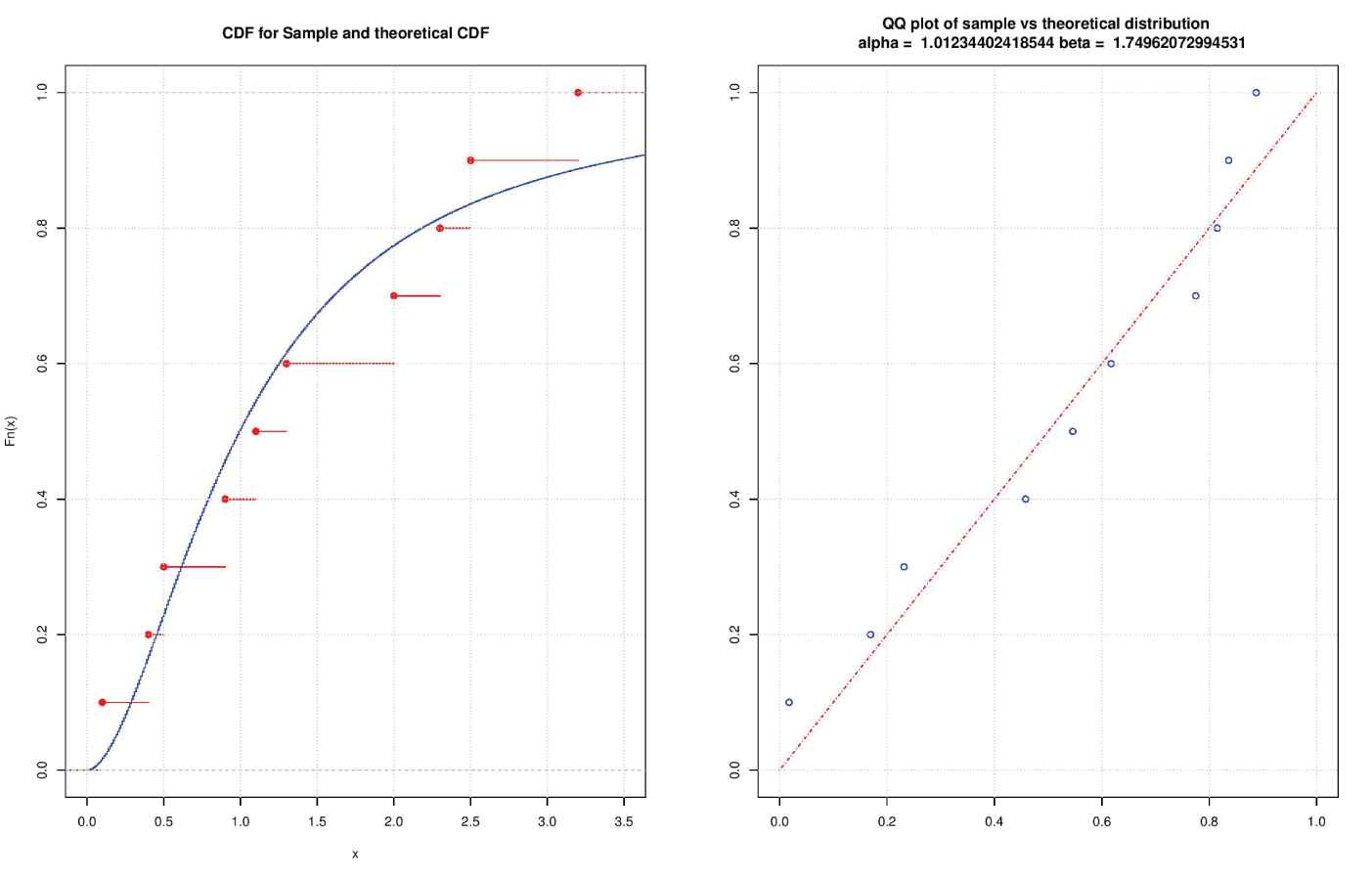
Expected Cumulative Distribution Function (ECDF) and Quintile-Quintile (Q-Q) plot of the real sample based on type-II exponentiated log-logistic (TIIELL) distribution.
Then by using the BLUEs coefficients in Tables 1 and 2, we have
| r | n | |||||||
|---|---|---|---|---|---|---|---|---|
| 1 | 1 | 0.166667 | 0.041667 | 0.013889 | 6.124244 | 24.00119 | 2.474721 | 21.00119 |
| 2 | 0.107379 | 0.015625 | 0.004095 | 1.480527 | 5.834856 | 1.216769 | 2.834856 | |
| 3 | 0.085248 | 0.009615 | 0.002348 | 0.970243 | 4.645654 | 0.985009 | 1.645654 | |
| 4 | 0.072834 | 0.006944 | 0.001639 | 0.775930 | 4.337018 | 0.880869 | 1.337018 | |
| 5 | 0.064627 | 0.005435 | 0.001258 | 0.690985 | 4.060399 | 0.831255 | 1.060399 | |
| 6 | 0.058687 | 0.004464 | 0.001020 | 0.653052 | 3.734868 | 0.808116 | 0.734868 | |
| 7 | 0.054132 | 0.003788 | 0.000858 | 0.577341 | 4.350134 | 0.759829 | 1.350134 | |
| 8 | 0.050495 | 0.003289 | 0.000739 | 0.576750 | 3.853975 | 0.759440 | 0.853975 | |
| 9 | 0.047505 | 0.002907 | 0.000650 | 0.534243 | 4.254706 | 0.730919 | 1.254706 | |
| 10 | 0.044990 | 0.002604 | 0.000580 | 0.479173 | 3.332768 | 0.692223 | 0.332768 | |
| 2 | 2 | 0.225955 | 0.067708 | 0.016652 | 6.669762 | 26.89585 | 2.582588 | 23.89585 |
| 3 | 0.151640 | 0.027644 | 0.004649 | 1.311287 | 5.810189 | 1.145115 | 2.810189 | |
| 4 | 0.122490 | 0.017628 | 0.002624 | 0.742933 | 4.483691 | 0.861936 | 1.483691 | |
| 5 | 0.105661 | 0.012983 | 0.001819 | 0.537407 | 4.080492 | 0.733081 | 1.080492 | |
| 6 | 0.094328 | 0.010287 | 0.001389 | 0.445519 | 3.949799 | 0.667472 | 0.949799 | |
| 7 | 0.086020 | 0.008523 | 0.001124 | 0.391159 | 3.375693 | 0.625427 | 0.375693 | |
| 8 | 0.079588 | 0.007277 | 0.000943 | 0.335838 | 3.046048 | 0.579516 | 0.046048 | |
| 9 | 0.074417 | 0.006349 | 0.000811 | 0.307304 | 3.904693 | 0.554350 | 0.904693 | |
| 10 | 0.070140 | 0.005632 | 0.000712 | 0.278758 | 3.848412 | 0.527975 | 0.848412 | |
| 3 | 3 | 0.263112 | 0.087740 | 0.018512 | 7.184192 | 28.97034 | 2.680334 | 25.97034 |
| 4 | 0.180790 | 0.037660 | 0.004975 | 1.322886 | 5.987013 | 1.150168 | 2.987013 | |
| 5 | 0.147734 | 0.024596 | 0.002771 | 0.707746 | 4.471739 | 0.841277 | 1.471739 | |
| 6 | 0.128326 | 0.018375 | 0.001907 | 0.492489 | 3.942891 | 0.701776 | 0.942891 | |
| 7 | 0.115099 | 0.014699 | 0.001451 | 0.380277 | 4.011283 | 0.616666 | 1.011283 | |
| 8 | 0.105315 | 0.012261 | 0.001170 | 0.312036 | 3.453741 | 0.558602 | 0.453741 | |
| 9 | 0.097688 | 0.010522 | 0.000979 | 0.302289 | 3.434712 | 0.549808 | 0.434712 | |
| 10 | 0.091521 | 0.009218 | 0.000842 | 0.251679 | 2.882750 | 0.501676 | 0.399884 | |
| 4 | 4 | 0.290553 | 0.104434 | 0.020013 | 7.578064 | 30.47057 | 2.752828 | 27.47057 |
| 5 | 0.202827 | 0.046370 | 0.005231 | 1.363788 | 6.098496 | 1.167813 | 3.098496 | |
| 6 | 0.167141 | 0.030817 | 0.002881 | 0.708859 | 4.536456 | 0.841938 | 1.536456 | |
| 7 | 0.145963 | 0.023276 | 0.001971 | 0.489885 | 3.966303 | 0.699918 | 0.966303 | |
| 8 | 0.131407 | 0.018762 | 0.001494 | 0.363963 | 3.895946 | 0.603293 | 0.895946 | |
| 9 | 0.120569 | 0.015738 | 0.001201 | 0.301321 | 3.393636 | 0.548927 | 0.393636 | |
| 10 | 0.112075 | 0.013565 | 0.001004 | 0.272530 | 3.072031 | 0.522044 | 0.072031 | |
| 5 | 5 | 0.312484 | 0.118950 | 0.021304 | 7.887611 | 31.61464 | 2.808489 | 28.61464 |
| 6 | 0.220670 | 0.054146 | 0.005451 | 1.404782 | 6.200086 | 1.185235 | 3.200086 | |
| 7 | 0.183024 | 0.036473 | 0.002975 | 0.717814 | 4.548271 | 0.847239 | 1.548271 | |
| 8 | 0.160518 | 0.027791 | 0.002025 | 0.477320 | 4.057296 | 0.690884 | 1.057296 | |
| 9 | 0.144955 | 0.022541 | 0.001529 | 0.368251 | 3.717102 | 0.606837 | 0.717102 | |
| 10 | 0.133308 | 0.018998 | 0.001227 | 0.293470 | 3.286510 | 0.541729 | 0.286501 | |
| 6 | 6 | 0.330847 | 0.131910 | 0.022450 | 8.139275 | 32.53265 | 2.852941 | 29.53265 |
| 7 | 0.235729 | 0.061216 | 0.005648 | 1.443160 | 6.280985 | 1.201316 | 3.280985 | |
| 8 | 0.196528 | 0.041682 | 0.003059 | 0.735319 | 4.529456 | 0.857508 | 1.529456 | |
| 9 | 0.172968 | 0.031990 | 0.002072 | 0.488891 | 4.037825 | 0.699208 | 1.037825 | |
| 10 | 0.156602 | 0.026085 | 0.001561 | 0.363625 | 3.532627 | 0.603013 | 0.532627 | |
| 7 | 7 | 0.346701 | 0.143693 | 0.023492 | 8.346127 | 33.28143 | 2.888966 | 30.28143 |
| 8 | 0.248795 | 0.067727 | 0.005828 | 1.477872 | 6.381171 | 1.215677 | 3.381171 | |
| 9 | 0.208308 | 0.046527 | 0.003135 | 0.750557 | 4.606563 | 0.866347 | 1.606563 | |
| 10 | 0.183879 | 0.035927 | 0.002116 | 0.499695 | 4.026693 | 0.706891 | 1.026693 | |
| 8 | 8 | 0.360687 | 0.154545 | 0.024450 | 8.522843 | 33.91907 | 2.919391 | 30.91907 |
| 9 | 0.260363 | 0.073784 | 0.005995 | 1.505565 | 6.457144 | 1.227015 | 3.457144 | |
| 10 | 0.218777 | 0.051071 | 0.003207 | 0.757008 | 4.664468 | 0.870062 | 1.664468 | |
| 9 | 9 | 0.373227 | 0.164640 | 0.025342 | 8.674506 | 34.46545 | 2.945251 | 31.46545 |
| 10 | 0.270760 | 0.079463 | 0.006152 | 1.531512 | 6.518105 | 1.237543 | 3.518105 | |
| 10 | 10 | 0.384613 | 0.174104 | 0.026177 | 8.808048 | 34.94389 | 2.967835 | 31.94389 |
Expected values, second moments, variances, skewness and kurtosis of the rth order statistic from type-II exponentiated log-logistic (TIIELL) distribution for
| r | n | |||||||
|---|---|---|---|---|---|---|---|---|
| 1 | 1 | 0.214757 | 0.062501 | 0.016379 | 1.482629 | 5.832059 | 1.217633 | 2.832059 |
| 2 | 0.145668 | 0.027778 | 0.006559 | 0.782284 | 4.113691 | 0.884468 | 1.113691 | |
| 3 | 0.117375 | 0.017857 | 0.004080 | 0.626158 | 3.790735 | 0.791301 | 0.790735 | |
| 4 | 0.100991 | 0.013158 | 0.002959 | 0.560859 | 3.566212 | 0.748905 | 0.566212 | |
| 5 | 0.089980 | 0.010417 | 0.002321 | 0.525832 | 3.442966 | 0.725143 | 0.442966 | |
| 6 | 0.081930 | 0.008621 | 0.001908 | 0.500077 | 3.502186 | 0.707161 | 0.502186 | |
| 7 | 0.075714 | 0.007353 | 0.001620 | 0.495238 | 3.237636 | 0.703732 | 0.237636 | |
| 8 | 0.070728 | 0.006410 | 0.001408 | 0.478453 | 3.227514 | 0.691703 | 0.227514 | |
| 9 | 0.066612 | 0.005682 | 0.001245 | 0.456279 | 3.397797 | 0.675484 | 0.397797 | |
| 10 | 0.063141 | 0.005102 | 0.001115 | 0.451449 | 3.303742 | 0.671901 | 0.303742 | |
| 2 | 2 | 0.283846 | 0.097222 | 0.016653 | 1.400052 | 6.014629 | 1.183238 | 3.014629 |
| 3 | 0.202256 | 0.047619 | 0.006712 | 0.563894 | 4.001324 | 0.750929 | 1.001324 | |
| 4 | 0.166526 | 0.031955 | 0.004224 | 0.391693 | 3.627183 | 0.625854 | 0.627183 | |
| 5 | 0.145032 | 0.024123 | 0.003089 | 0.322388 | 3.480211 | 0.567792 | 0.480211 | |
| 6 | 0.130231 | 0.019397 | 0.002437 | 0.284753 | 3.357070 | 0.533623 | 0.357070 | |
| 7 | 0.119225 | 0.016227 | 0.002012 | 0.265080 | 3.246232 | 0.514859 | 0.246232 | |
| 8 | 0.110621 | 0.013952 | 0.001715 | 0.245458 | 3.320959 | 0.495437 | 0.320959 | |
| 9 | 0.103652 | 0.012238 | 0.001494 | 0.230641 | 3.469610 | 0.480251 | 0.469610 | |
| 10 | 0.097858 | 0.010901 | 0.001324 | 0.233139 | 2.927740 | 0.482845 | 0.218501 | |
| 3 | 3 | 0.324642 | 0.122024 | 0.016632 | 1.466340 | 6.256670 | 1.210925 | 3.256670 |
| 4 | 0.237985 | 0.063283 | 0.006646 | 0.526732 | 4.039598 | 0.725763 | 1.039598 | |
| 5 | 0.198768 | 0.043703 | 0.004194 | 0.342041 | 3.552107 | 0.584842 | 0.552107 | |
| 6 | 0.174635 | 0.033575 | 0.003078 | 0.263913 | 3.429646 | 0.513725 | 0.429646 | |
| 7 | 0.157746 | 0.027320 | 0.002436 | 0.222956 | 3.410097 | 0.472182 | 0.410097 | |
| 8 | 0.145037 | 0.023054 | 0.002018 | 0.193353 | 3.346856 | 0.439719 | 0.346856 | |
| 9 | 0.135010 | 0.019951 | 0.001723 | 0.176914 | 3.377494 | 0.420612 | 0.377494 | |
| 10 | 0.126829 | 0.017590 | 0.001504 | 0.175914 | 2.934875 | 0.419421 | 0.192158 | |
| 4 | 4 | 0.353527 | 0.141604 | 0.016623 | 1.540551 | 6.459855 | 1.241189 | 3.459855 |
| 5 | 0.264129 | 0.076337 | 0.006573 | 0.522017 | 4.094437 | 0.722507 | 1.094437 | |
| 6 | 0.222901 | 0.053831 | 0.004146 | 0.322694 | 3.617912 | 0.568062 | 0.617912 | |
| 7 | 0.197152 | 0.041916 | 0.003047 | 0.241729 | 3.378629 | 0.491659 | 0.378629 | |
| 8 | 0.178928 | 0.034431 | 0.002416 | 0.197982 | 3.283768 | 0.444952 | 0.283768 | |
| 9 | 0.165092 | 0.029259 | 0.002004 | 0.179578 | 3.085929 | 0.423766 | 0.085929 | |
| 10 | 0.154098 | 0.025460 | 0.001714 | 0.161099 | 3.196057 | 0.401371 | 0.196057 | |
| 5 | 5 | 0.375877 | 0.157921 | 0.016637 | 1.608648 | 6.618557 | 1.268325 | 3.618557 |
| 6 | 0.284744 | 0.087590 | 0.006511 | 0.529866 | 4.110246 | 0.727919 | 1.110246 | |
| 7 | 0.242213 | 0.062767 | 0.004101 | 0.317573 | 3.609708 | 0.563536 | 0.609708 | |
| 8 | 0.215376 | 0.049401 | 0.003014 | 0.232813 | 3.364292 | 0.482507 | 0.364292 | |
| 9 | 0.196223 | 0.040895 | 0.002392 | 0.189503 | 3.326950 | 0.435320 | 0.326950 | |
| 10 | 0.181583 | 0.034958 | 0.001986 | 0.166596 | 3.238532 | 0.408162 | 0.238532 | |
| 6 | 6 | 0.394104 | 0.171987 | 0.016669 | 1.668102 | 6.757334 | 1.291550 | 3.757334 |
| 7 | 0.301756 | 0.097519 | 0.006462 | 0.540625 | 4.142795 | 0.735272 | 1.142795 | |
| 8 | 0.258315 | 0.070787 | 0.004060 | 0.313873 | 3.650085 | 0.560244 | 0.650085 | |
| 9 | 0.230698 | 0.056205 | 0.002983 | 0.229549 | 3.451351 | 0.479112 | 0.451351 | |
| 10 | 0.210864 | 0.046832 | 0.002368 | 0.180792 | 3.353638 | 0.425196 | 0.353638 | |
| 7 | 7 | 0.409495 | 0.184398 | 0.016712 | 1.719701 | 6.877223 | 1.311373 | 3.877223 |
| 8 | 0.316236 | 0.106430 | 0.006425 | 0.551682 | 4.167832 | 0.742753 | 1.167832 | |
| 9 | 0.272123 | 0.078077 | 0.004026 | 0.318976 | 3.677382 | 0.564780 | 0.677382 | |
| 10 | 0.243921 | 0.062454 | 0.002957 | 0.228410 | 3.391861 | 0.477923 | 0.391861 | |
| 8 | 8 | 0.422818 | 0.195537 | 0.016762 | 1.764809 | 6.979383 | 1.328461 | 3.979383 |
| 9 | 0.328840 | 0.114530 | 0.006394 | 0.562789 | 4.217233 | 0.750193 | 1.217233 | |
| 10 | 0.284209 | 0.084773 | 0.003998 | 0.320279 | 3.693316 | 0.565932 | 0.693316 | |
| 9 | 9 | 0.434565 | 0.205663 | 0.016816 | 1.805957 | 7.064301 | 1.343859 | 4.064301 |
| 10 | 0.339998 | 0.121970 | 0.006371 | 0.572928 | 4.244680 | 0.756920 | 1.244680 | |
| 10 | 10 | 0.445072 | 0.214962 | 0.016873 | 1.842618 | 7.141398 | 1.357431 | 4.141398 |
Expected values, second moments, variances, skewness and kurtosis of the rth order statistic from type-II exponentiated log-logistic (TIIELL) distribution for
| 90% CI | 95% CI | |
|---|---|---|
| Edgeworth | (0.6257, 1.13836) | (0.27096, 1.14393) |
| Simulated | (0.6275, 1.23062) | (0.48281, 1.24881) |
By using Table 8, the CIs for the location parameter
| 90% CI | 95% CI | |
|---|---|---|
| Edgeworth | (0.99163, 3.59568) | (1.00122, 3.65746) |
| Simulated | (1.02546, 3.59603) | (0.91974, 3.67228) |
By using Table 10, the CIs for the scale parameter
| 90% CI | 95% CI | |
|---|---|---|
| Simulated | (0.56691, 2.91362) | (0.48181, 3.54143) |
By using Table 10, the CIs for the location parameter
We note that the average width of the CIs increase as the level of significant increases.
7. CONCLUSION
In this paper, the moments and product moments of the order statistics from the TIIELL distribution are derived in explicit forms. The single and double moments are used to obtain the BLUEs of the location and scale parameters of TIIELL distribution. The variances and covariances are calculated to show the performance of the BLUEs. Next, we calculate mean, variance, coefficient of skewness and kurtosis for some linear pivotal quantities. The distributions of the pivotal quantities are calculated in terms of Edgeworth approximation based on BLUEs which in turn can be used to develop CIs. Hence, the distributions of the pivotal quantities are used to construct the interval estimation for the location and scale parameters. The accuracy of the estimated CIs is investigated in terms of the average width. Finally, one real data set has been used to obtain the MLEs of the model parameters, BLUEs of
CONFLICTS OF INTEREST
The authors declare that there are no conflicts of interest regarding the publication of this paper.
AUTHORS' CONTRIBUTIONS
All authors contributed equally to the writing of this paper. All authors have read and agreed to the published version of the manuscript.
FUNDING STATEMENT
There is no funding of this paper.
ACKNOWLEDGMENTS
The authors would like to express thanks to the editor and anonymous referees for useful suggestions and comments which have improved the presentation of the manuscript.
REFERENCES
Cite this article
TY  - JOUR
AU  - Devendra Kumar
AU  - Maneesh Kumar
AU  - Sanku Dey
PY  - 2020
DA  - 2020/09/11
TI  - Inferences for the Type-II Exponentiated Log-Logistic Distribution Based on Order Statistics with Application
JO  - Journal of Statistical Theory and Applications
SP  - 352
EP  - 367
VL  - 19
IS  - 3
SN  - 2214-1766
UR  - https://doi.org/10.2991/jsta.d.200825.002
DO  - 10.2991/jsta.d.200825.002
ID  - Kumar2020
ER  -