
On Examining Complex Systems Using the q-Weibull Distribution in Classical and Bayesian Paradigms

- DOI
- 10.2991/jsta.d.200825.001How to use a DOI?
- Keywords
- Bayesian analysis; MCMC simulations; ML estimation; Model selection criteria; Posterior estimates; q-Weibull distribution
- Abstract
The q-Weibull distribution is a generalized form of the Weibull distribution and has potential to model complex systems and life time datasets. Bayesian inference is the modern statistical technique that can accommodate uncertainty associated with the model parameters in the form of prior distributions. This study presents Bayesian analysis of the q-Weibull distribution using uninformative and informative priors and the results are compared with those produced by the classical maximum likelihood (ML) and least-squares (LS) estimation methods. A simulation study is also made to compare the competing methods. Different model selection criteria and predicted datasets are considered to compare the inferential methods under study. Posterior analyses include evaluating posterior means, medians, credible intervals of highest density regions, and posterior predictive distributions. The entire analysis is carried out using Markov chain Monte Carlo (MCMC) setup using WinBUGS package. The Bayesian method has proved to be superior to its classical counterparts. A real dataset is used to illustrate the entire inferential procedure.
- Copyright
- © 2020 The Authors. Published by Atlantis Press B.V.
- Open Access
- This is an open access article distributed under the CC BY-NC 4.0 license (http://creativecommons.org/licenses/by-nc/4.0/).
1. INTRODUCTION
Several q-type distributions are proposed to model complex systems appearing in the fields of biology, chemistry, economics, geography, informatics, linguistics, mathematics, medicine, physics, etc. [1–3]. The q-type distributions are based on functions that are used in nonextensive statistical mechanics of nonextensive formalism [4].
Depending upon the importance of these distributions, a variety of q-type distributions has been suggested to model several phenomena. Most important being q-exponential [1,5–7], q-gamma [6], q-Gaussian [1], and q-Weibull [1,5–8]. A good discussion on the q-Weibull distribution and its applications may be seen in [9]. Besides modeling the complex systems, the q-W distribution also has the potential to describe lifetime datasets [4,10–13]. Therefore, it has got much popularity and is frequently used in different fields.
Classical methods are frequently used in the analysis but they suffer from a certain drawbacks. The frequentists consider parameters to be unknown fixed quantities and they just rely on current datasets and deprive the results of any prior information available about the parameters of interest. Whereas, the parameters are assumed random quantities in the Bayesian approach and hence follow certain probability distribution and take both the current dataset and prior information about the parameters into account. As a result, we get a posterior distribution that is believed to average the current dataset and the prior information, and is hence used for all types of subsequent inference. A good review and advantages of using Bayesian methods may be found in [10,12,14–20]. The posterior distributions often have complex multidimensional forms that require using Markov chain Monte Carlo (MCMC) methods to get results [15,21–24]. In recent years, the use of MCMC methods has gained much popularity [25,26,27].
It has now been established that the q-Weibull distribution is a good choice to model complex systems and lifetime datasets appearing in a variety of fields. The probability density function (pdf) of the q-Weibull distribution is given as
And the cumulative distribution function (CDF) is
Here
Due to variety of applications of the q-Weibull distribution, the efficient estimation of the PDF and the CDF of the q-Weibull distribution is the purpose of the present study. Jia et al. [4] have recently worked out the classical maximum likelihood (ML) and least-square (LS) estimators for the q-Weibull distribution. We have analyzed the q-Weibull distribution in Bayesian framework to avail the aforesaid advantages the approach.
2. THE FREQUENTIST APPROACH OF STATISTICAL ANALYSIS
Two alternative probabilistic methods—the frequentist classical and the Bayesian methods—are proposed and used in data analyses. We estimate the parameters of the q-Weibull distribution using both the frequentist and the Bayesian methods. In statistical terminology, the data generating process of any system depends on the system-specific characteristics, called parameters. So the dataset being generated from the model is believed to follow and exhibit the impact of parameters. The uncertainty associated with the data values is defined in terms of frequencies of the data values generating from the system under study. It is considered as the default approach to be used in variety of areas of sciences. Commonly used frequentist methods of statistical inference include uniformly minimum variance unbiased, ML, percentile, LS, weighted LS methods, etc. But we just report the most commonly used ML and LS estimation method whose results will henceforth be compared with their Bayesian counterparts. Here we will just confine ourselves to report the results already produced by [4].
2.1. Maximum Likelihood Estimation
The likelihood function gives the probability of the observed sample generated by the model, system, or distribution under study. The ML estimation professed by [28] calls for choosing those values of the parameters that maximize the probability of the very observed sample. We generally opt for algebraic maximization of the likelihood function to find the ML estimates, but we may also opt for evaluating the probabilities of the observed samples at all possible values of the parameters and to choose those parametric values as the ML estimates that maximize the evaluated probabilities of the observed samples. However, for the algebraic maximization to find the ML estimates, we proceed as follows:
Let
Taking logarithm, we get
The first derivatives of the log-likelihood
Equating them to zero gives us the normal equations to be solved for the ML estimates. As these equations are nonlinear, so we cannot get their closed forms and will need numerical methods to solve them. We have used “optim” function of R package to get these estimates. For more details on the estimation of the q-Weibull distribution, please refer to [4].
3. THE BAYESIAN APPROACH OF STATISTICAL ANALYSIS
A brief overview on this topic is already given in Section 1. Bayesian method combines prior information about the model parameters with dataset using Bayes rule yielding the posterior distribution. The Bayes rule is named after Thomas Bayes, whose work on this topic was published in 1763, two years after his death [29].
To establish Bayesian inference set-up, we need a model or system in the form of a probability distribution controlled by a set of parameters to be estimated, the sample dataset generated by the model or distribution, and a prior distribution based on the prior knowledge of experts regarding the parameters of interest. These elements are formally combined in to posterior distribution which is regarded as a key-distribution and work-bench for the subsequent analyses. The algorithm is explained in Figure 1.
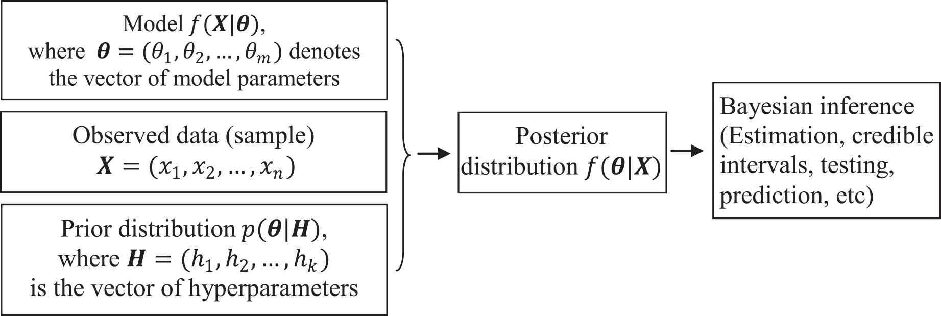
Flowchart of the Bayesian procedure for inference of parameters.
If
The denominator is independent of model parameters
4. THE PRIOR DISTRIBUTIONS
It has already been elaborated that main difference between classical and Bayesian approaches is to use prior information regarding the model parameters in the analysis. The formal way of doing so it to quantify the knowledge of experts into a prior distribution that can adequately fit to the nature of the parameter and the experts’ opinion. The parameters of the prior distribution, known as hyperparameters, are elicited in the light of the subjective expert opinion. So, the prior has a leading role in the analysis, and hence must be selected and elicited very carefully. It may be misleading, otherwise.
4.1. Uninformative Priors
When there is lack of knowledge about the model parameters, we prefer to choose vague, defuse, or flat priors. As the q-Weibull distribution is based on the set of parameters
4.2. Informative Priors
When there is sufficient information available about the model parameters, then it becomes necessary to avail it by assigning informative priors to the model parameters such that they can adequately fit to the knowledge available for the model parameters being examined. In the present situation, we observe that the parameters
Here again
It is important to notice that the experts may not be the experts of statistics and hence cannot translate their expertise in statistical terms. So it is the sole responsibility of the statisticians to formally utilize the experts’ prior information and elicit the values of the hyperparameters of the prior density which are to be subsequently used in the Bayesian analysis. Elicitation of hyperparameters is beyond the scope of our study. However, an exhaustive discussion on the elicitation of hyperparameters may be found in [30]. We will, however, proceed just by carefully choosing the values of the hyperparameters to be used in the Bayesian analysis.
4.3. The Posterior Distribution
Being specific to estimation of the parameters of q-Weibull distribution, let the vector of parameters of interest and the dataset are denoted by
The marginal posterior distributions
4.4. Bayes Estimates
To work out the Bayes estimates of the parameters
The marginal posterior distributions are generally of complicated nature and hence are evaluated by numerical methods. Markov Chains Monte Carlo (MCMC) is the most frequently used numerical method to be used in Bayesian inference. So we also proceed with MCMC with the WinBUGS package to find the posterior summaries of the parameters of interest.
5. THE MARKOV CHAIN SIMULATIONS
To compare the performance of the ML and Bayes estimates, the Markov Chain (MC) simulation study is made for different values of the parameters and sample of sizes 50, 100, 200, 400, 800, and 100. The process is repeated for 10000 times for every combination of the parameters. The ML estimates, their standard errors and confidence intervals (CIs) are constructed and the results in terms of relative bias, relative mean square errors (MSEs), and relative length of CI are presented in Figure 2. Here we observed to obtain a little amount of relative bias, relative MSEs, and relative lengths of CI for all combinations of parameter values, which further decease by increasing the sample size. A similar MC simulation study is also made to evaluate the Bayes estimates.
As we know that in Bayes estimation, parameters are considered random variable and we evaluate Bayes estimates under different loss function on the entire range of the parameters. We also draw marginal posterior distributions that are based on the entire support of the parameters. Hence Bayes estimates are considered unbiased. In the simulation study, we have also observed and verified this property. Further studies of MCMC simulations are performed using the real-life dataset and the results are presented in Section 6.
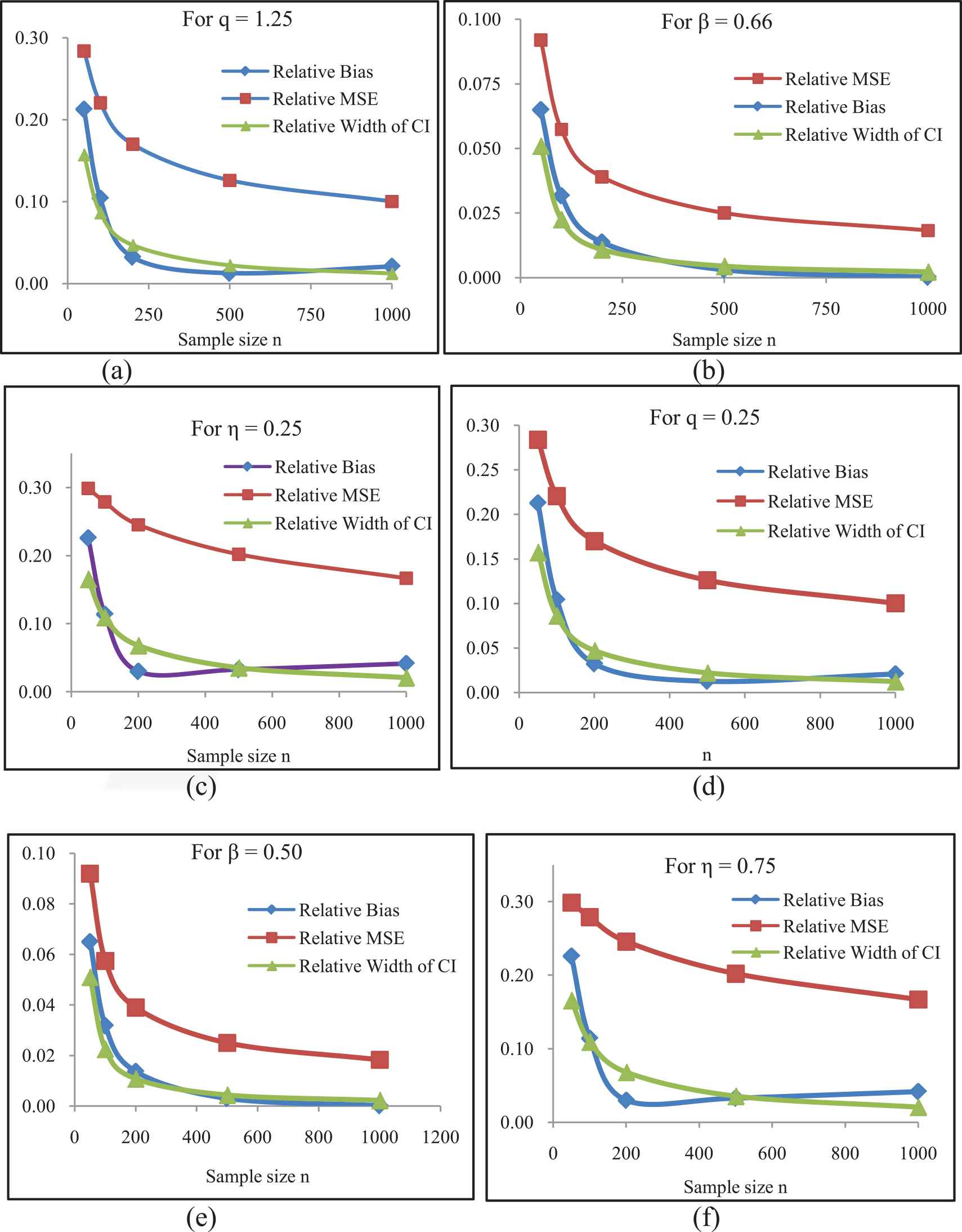
Comparison of relative bias, mean square error (MSE) and width of confidence intervals for the maximum likelihood (ML) estimates of the parameters q (a, d), β (b, e), and η (c, f) for increasing n.
5.1. Illustrative Example
Let us consider the real dataset for the q-Weibull distribution that represent time to failure for a group of 36 generators of 500 MW [31], is used. The dataset comprises 0.058, 0.070, 0.090, 0.105, 0.113, 0.121, 0.153, 0.159, 0.224, 0.421, 0.570, 0.596, 0.618, 0.834, 1.019, 1.104, 1.497, 2.027, 2.234, 2.372, 2.433, 2.505, 2.690, 2.877, 2.879, 3.166, 3.455, 3.551, 4.378, 4.872, 5.085, 5.272, 5.341, 8.952, 9.188, and 11.399 (1000’s of hours). The summary of the dataset is presented in Table 1 along with its figurative representation made in Figures 3–5.
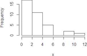
Histogram of the observed dataset.
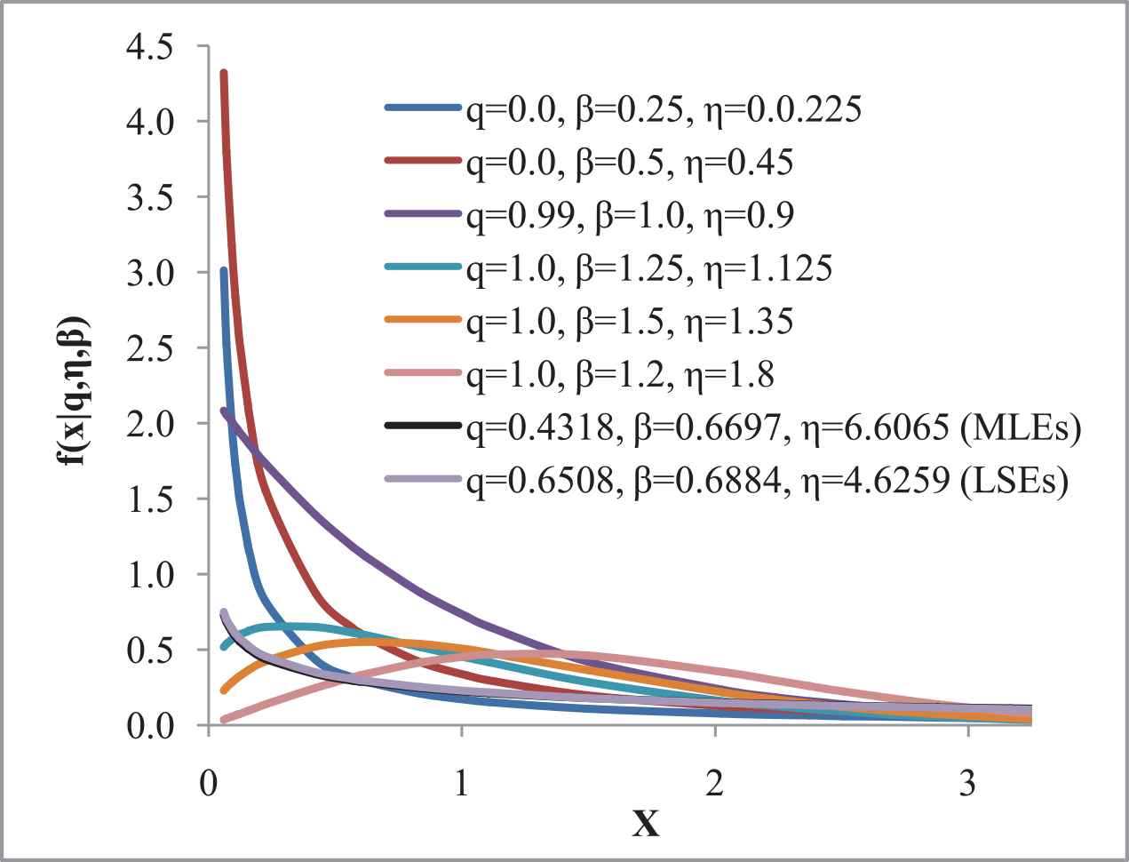
Probability density functions (PDFs) of q-Weibull distribution at different parametric values the observed data points.
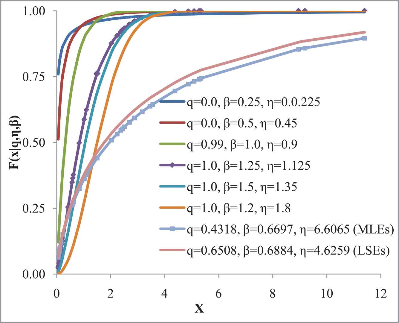
Cumulative distribution function (CDFs) of q-Weibull distribution at different parametric values the observed data points.
Obviously, the observed dataset is positively skewed. As stated in Section 2.1, the normal equations we get using the observed dataset are complicated and hence the estimates are found using the numerical methods. Following [4], the ML estimates, LS estimates, and 95 % CIs for the parameters are reported in Table 2.
| Min. | 1st Qu. | Median | Mean | 3rd Qu. | Max. |
|---|---|---|---|---|---|
| 0.058 | 0.3718 | 2.1305 | 2.5674 | 3.479 | 11.399 |
Summary of the observed dataset.
| Parameters | MLEs | LSEs | 95% Confidence Intervals |
|---|---|---|---|
| 0.4318 | 0.6508 | (1.8999; 2.6761) | |
| 0.6697 | 0.6884 | (0.6290; 0.7230) | |
| 0.2824 | 0.3484 | (0.6030; 0.7010) |
Note: MLE, maximum likelihood estimation; LSE, least square estimation.
The MLEs, LSEs, standard error, and 95% confidence intervals.
6. THE MCMC METHOD
The MCMC method selects random sample from the (posterior) probability distribution according to random process termed as MCs, where every new step of the process depends on the current state and is completely independent of previous states. The MCMC method can be implemented using any of the standard softwares like R, Python, etc., but the most specific software being used for the Bayesian analysis is Windows based Bayesian inference Using Gibbs Sampling (WinBUGS). We didn’t specify the initial values of the hyperparameters and let the WinBUGS choose them by itself, and generated 20,000 values following a burn-in of 10,000 iterations. The WinBUGS codes used to analyze the dataset are given in Appendix for the readers to follow.
6.1. Bayesian Analyses Using Uninformative Uniform Priors
Assuming the uniform priors for all the set of parameters under study as defined in Section 4.1, the WinBUGS codes are run and the resulting Bayes estimates, standard errors, medians, and 95% credible intervals of highest density regions along with the associated values of the hyperparameters are presented in Table 3.
| Uninformative Uniform Priors | Parameters | Means | SEs | MC Error | Medians | 95% Credible Intervals |
|---|---|---|---|---|---|---|
| 0.4503 | 0.2615 | 0.0025 | 0.4463 | (0.0225; 0.8786) | ||
| 0.7544 | 0.4347 | 0.0041 | 0.7557 | (0.0392; 1.4640) | ||
| 2.9870 | 1.7380 | 0.0171 | 2.9600 | (0.1472; 5.8530) | ||
| 0.3002 | 0.1743 | 0.0016 | 0.2976 | (0.0150; 0.5857) | ||
| 0.7544 | 0.4347 | 0.0041 | 0.7557 | (0.0392; 1.4640) | ||
| 2.9870 | 1.7380 | 0.0171 | 2.9600 | (0.1472; 5.8530) | ||
| 0.2502 | 0.1453 | 0.0014 | 0.2480 | (0.0125; 0.4881) | ||
| 0.7544 | 0.4347 | 0.0041 | 0.7557 | (0.0392; 1.4640) | ||
| 2.9870 | 1.7380 | 0.0171 | 2.9600 | (0.1472; 5.8530) | ||
| 0.1251 | 0.0727 | 0.0007 | 0.1240 | (0.0062; 0.2441) | ||
| 0.7544 | 0.4347 | 0.0041 | 0.7557 | (0.0392; 1.4640) | ||
| 2.9870 | 1.7380 | 0.0171 | 2.9600 | (0.1472; 5.8530) | ||
| 0.0500 | 0.0291 | 0.0003 | 0.0496 | (0.0025; 0.0976) | ||
| 0.7544 | 0.4347 | 0.0041 | 0.7557 | (0.0392; 1.4640) | ||
| 2.9870 | 1.7380 | 0.0171 | 2.9600 | (0.1472; 5.8530) | ||
| 0.0500 | 0.0291 | 0.0003 | 0.0496 | (0.0025; 0.0976) | ||
| 0.8544 | 0.4347 | 0.0041 | 0.8557 | (0.1392; 1.5640) | ||
| 2.4890 | 1.4480 | 0.0143 | 2.4670 | (0.1227; 4.8780) |
Note: MC, Markov chain.
Summary of Bayes estimates under the uninformative uniform priors.
It is observed that the elicited hyperparameters have high impact on the Bayes estimates. The initial values have no significant effects on the posterior estimates if the true convergence is achieved.
6.2. Bayesian Analyses Using Informative Uniform-Gamma Priors
As already discussed that the Bayesians use prior information shared by the field experts about the unknown parameters in the analysis; so, we assume the uniform-gamma priors for the set of model parameters under study as defined in Section 4.2. We have carefully chosen the values of the hyperparameters and the WinBUGS codes are again run for 20,000 iterations following 10,000 iterations as burn-in. The resulting Bayes estimates, standard errors, medians, and 95% credible intervals of highest density regions along with the associated values of the hyperparameters are presented in Table 4.
It is again observed that the elicited hyperparameters have high impact on the Bayes estimates. The initial values have no significant effect on the posterior estimates if the convergence in MC is achieved.
| Uniform-Gamma Priors | Parameters | Means | SEs | MC Error | Medians | 95% Credible Intervals |
|---|---|---|---|---|---|---|
| 0.0501 | 0.0289 | 0.0003 | 0.0505 | (0.0025; 0.0976) | ||
| 0.8024 | 0.8999 | 0.0090 | 0.4974 | (0.0083; 3.2420) | ||
| 2.4280 | 4.9780 | 0.0463 | 0.3599 | (0.0000; 17.1700) | ||
| 0.0500 | 0.0290 | 0.0002 | 0.0499 | (0.0023; 0.0974) | ||
| 0.7940 | 0.8917 | 0.0062 | 0.4942 | (0.0091; 3.2040) | ||
| 2.3610 | 3.9420 | 0.0285 | 0.7527 | (0.0002; 14.0100) | ||
| 0.9935 | 0.5772 | 0.0056 | 0.9888 | (0.0487; 1.9510) | ||
| 0.8050 | 0.8990 | 0.0084 | 0.4998 | (0.0083; 3.2900) | ||
| 2.4160 | 4.0750 | 0.0380 | 0.7477 | (0.0002; 14.2300) | ||
| 0.4511 | 0.1732 | 0.0013 | 0.4509 | (0.1666; 0.7356) | ||
| 0.6764 | 0.5992 | 0.0041 | 0.5162 | (0.0320; 2.2540) | ||
| 6.4520 | 4.3140 | 0.0289 | 5.5280 | (0.9479; 17.3900) | ||
| 0.1741 | 0.0434 | 0.0004 | 0.1737 | (0.1038; 0.2462) | ||
| 0.0809 | 0.2094 | 0.0022 | 0.0037 | (0.0000; 0.6930) | ||
| 2.3980 | 4.0530 | 0.0457 | 0.7484 | (0.0002; 14.310) | ||
| 0.0150 | 0.0029 | 0.0000 | 0.0150 | (0.0103; 0.0198) | ||
| 0.8223 | 0.7359 | 0.0075 | 0.6123 | (0.0385; 2.7430) | ||
| 2.3120 | 1.8860 | 0.0200 | 1.8120 | (0.1791; 7.1990) |
Note: MC, Markov chain.
Summary of Bayes estimates under the informative uniform-gamma priors.
6.3. Convergence Diagnostics
Sequential plots are used in WinBUGS to assess difficulties in MCMC and realization of the model. In MCMC simulations, the values of the parameters of interest are sampled from the posterior distributions. So the estimates will be convergent if the posterior distributions are stationary in nature and the MC will seem to be mixing well. To check convergence, different graphical representations of parametric behavior are used in MCMC implemented through WinBUGS.
6.3.1. History time series plots
The time series history plots of parameters are presented in Figure 6. Here, MC seems to be mixing well enough and is being sampled from the stationary distribution. The plots are in the form of horizontal bands with no extraordinary upward or downward trends. It indicates that the MChas converged.
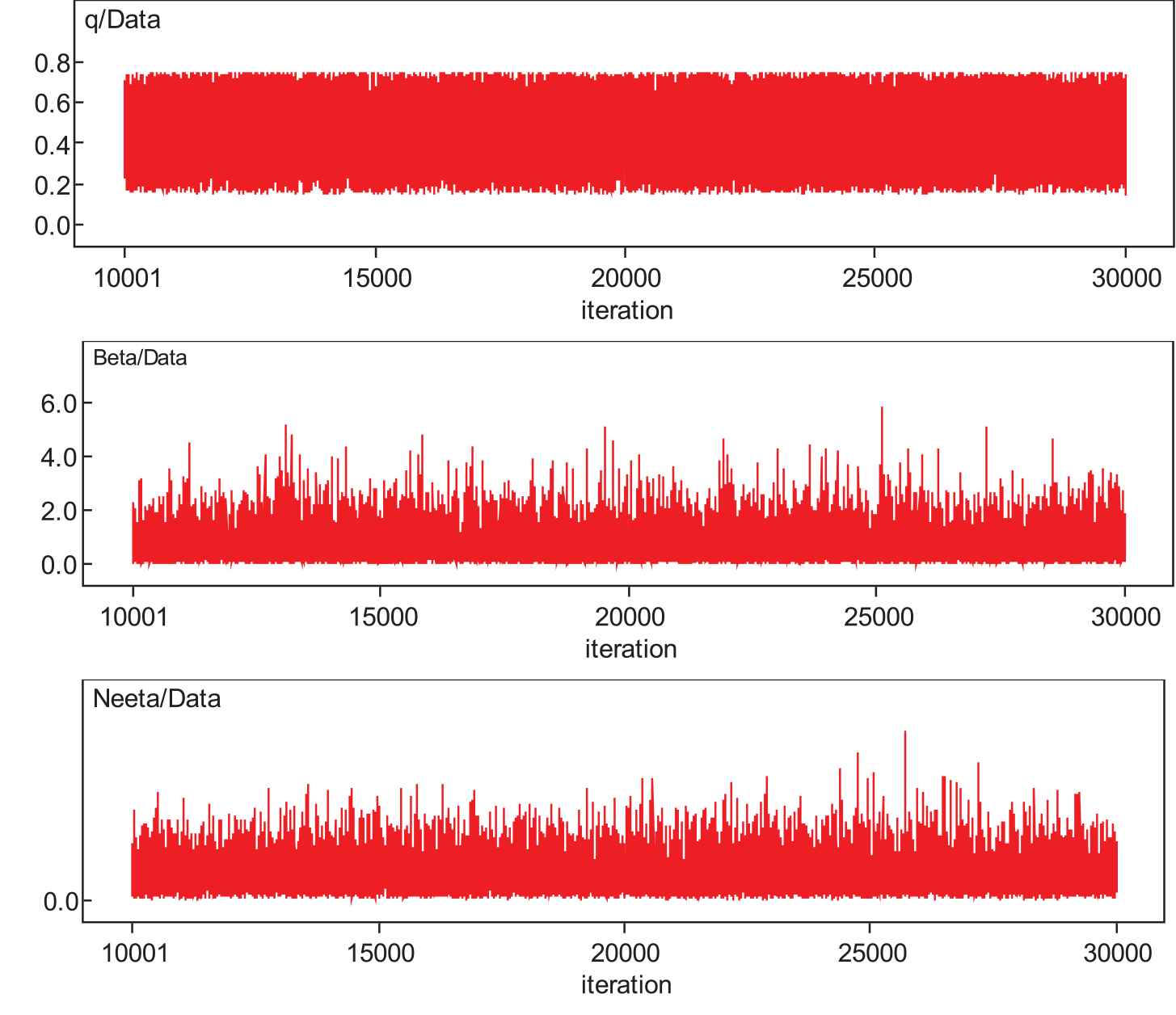
Time series plots of the parameters .
6.3.2. Dynamic traces and autocorrelation function
The traces of the parameters and autocorrelation graphs of
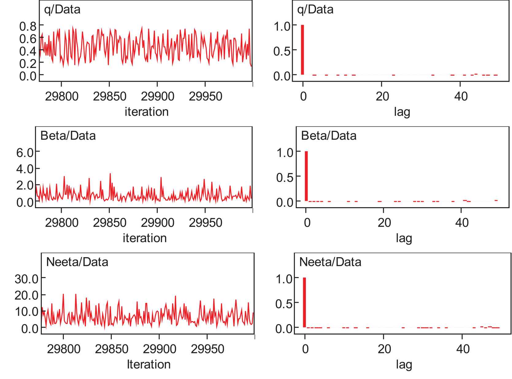
Dynamic traces and autocorrelation function.
6.3.3. Some other graphical representations
Proper density expressed without normalizing constant are termed as the kernel densities. They may exhibit the symmetry, kurtosis, and general behavior of the distribution. Kernel density plots, running quantiles, and box plots based on the posterior densities of the parameters are presented in Figure 8.
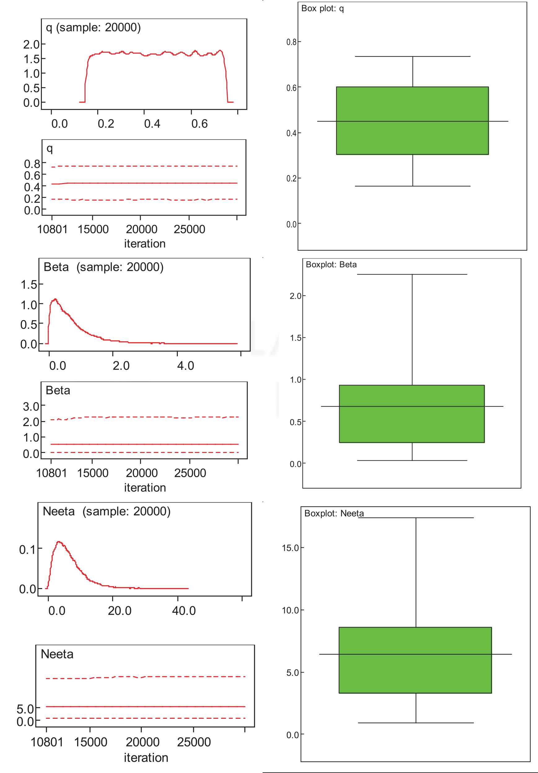
Posterior densities, running quantiles, and box plots of marginal posterior densities of the model parameters.
Obviously, the posterior marginal densities of
6.4. Predictive Inference
After finding out the Bayes estimates, it is necessary to evaluate them and to compare them with their classical counterparts based on the predictive inference. Suppose that the models
As we have the original dataset of 36 observations, so predicted samples of the same size, i.e., 36 observations, is generated based on the ML, LS, and Bayes estimates. The predicted dataset along with their summaries are presented in Table 5 and Figure 9.
| Data Types | Min | Median | Max | Mean | SD | 95% C. Limits | ||
|---|---|---|---|---|---|---|---|---|
| Observed dataset | 0.0580 | 0.3718 | 2.1305 | 3.4790 | 11.3990 | 2.5674 | 7.8329 | (1.6532; 3.4817) |
| Predicted by MLE | 0.0050 | 0.8431 | 1.4160 | 2.9952 | 9.6573 | 2.5395 | 7.4042 | (1.6506; 3.4284) |
| Predicted by LSE | 0.0053 | 0.8016 | 1.4160 | 2.8871 | 10.4101 | 2.5395 | 7.4042 | (1.6506; 3.4284) |
| Predicted by Bayes | 0.0054 | 0.8578 | 1.4160 | 3.0211 | 9.7324 | 2.5395 | 7.4042 | (1.6506; 3.4284) |
Note: MLE, maximum likelihood estimation; LSE, least square estimation.
Summary of the observed and predicted datasets based on MLE, LSE, and Bayes estimates.
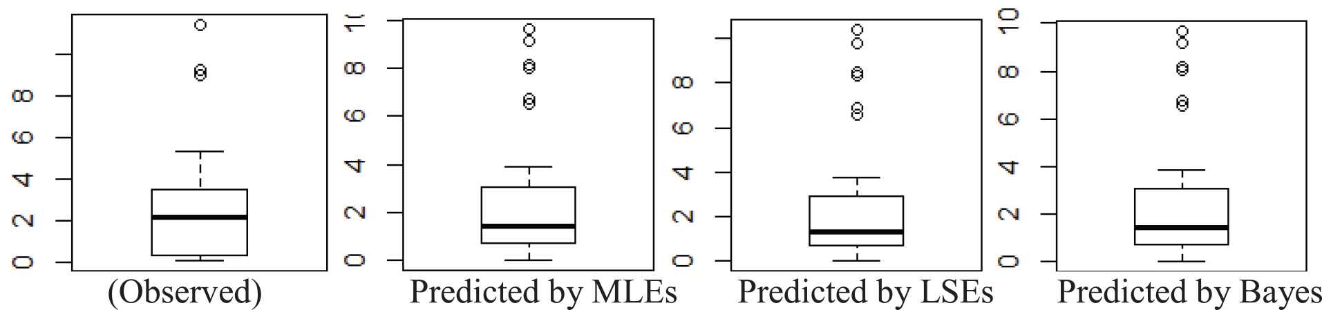
Boxplots of observed and predicted/expected datasets under maximum likelihood estimations (MLEs), least-squares estimations (LSEs), and Bayes estimates.
It is very much interesting to note that the summary of the estimates produced by the original observed dataset agree with those produced by future predicted datasets based on the ML, LS, and Bayes estimates. Moreover, the summaries of the future datasets predicted by three major competing approaches, i.e., the ML estimation, LSE, and Bayesian estimation fully agree with each other. So it may be claimed that Bayes methods are the potential candidates to be used in any inferential procedures used in any field knowledge.
7. COMPARISON OF THE FREQUENTIST AND BAYESIAN APPROACHES
An important aspect of this study is to compare the Bayes estimation methods with the classical counterparts. Such comparisons may be made on the basis of the posterior predictive inference and the model selection criteria. It is of prime interest to note that the posterior predictive inference presented in Section 6.4 plays a dual role in inference. Firstly, it can predict the future observations of the data, and secondly, it has the potential to offer a strong basis for the comparison of different models and estimate methods. We have witnessed its comparison role in Section 6.4.
7.1. Model Selection Criteria
The classical and Bayesian estimation methods can also be compared using the model selection criteria [32]. So we use pure ML, Akaike information criterion (AIC), corrected AIC (AICC), Bayes information criterion (BIC, also known as Schwarz criterion), and Hannan–Quinn criterion (HQC), which are respectively defined as
Here
Here we observe from the values of model selection criteria produced by the ML, LS, uninformative Bayes, and informative Bayes methods that all the five criteria stated above yield smaller values for the Bayes methods. These values get even smaller if we go on changing the values of the hyperparameters. However, it is pertinent to note that these results are sensitive to the selection of the values of the hyperparameters. Hence, a careful choice or elicitation of the hyperparameters is demanding and to produce ideal results by using the Bayesian methods. Carefully selected or elicited values of the hyperparameters may lead to even better values of the model selection criteria.
| Estimation Methods | Estimates of |
Log-likelihood | ML | AIC | AICC | BIC | HQC | ||
|---|---|---|---|---|---|---|---|---|---|
| MLEs | 0.432 | 6.607 | 0.670 | −61.810 | 123.620 | 129.620 | 130.370 | 134.371 | 127.449 |
| LSEs | 0.651 | 4.626 | 0.688 | −62.979 | 125.958 | 131.958 | 132.708 | 136.708 | 129.787 |
| Uninformative Bayes estimates | 0.450 | 2.987 | 0.754 | −53.911 | 107.821 | 113.821 | 114.571 | 118.572 | 111.650 |
| 0.300 | 2.987 | 0.754 | −50.582 | 101.165 | 107.165 | 107.915 | 111.915 | 104.994 | |
| 0.250 | 2.987 | 0.754 | −49.539 | 99.077 | 105.077 | 105.827 | 109.828 | 102.906 | |
| 0.125 | 2.987 | 0.754 | −47.053 | 94.106 | 100.106 | 100.856 | 104.856 | 97.935 | |
| 0.050 | 2.987 | 0.754 | −45.639 | 91.279 | 97.279 | 98.029 | 102.029 | 95.108 | |
| 0.050 | 2.489 | 0.854 | −44.743 | 89.486 | 95.486 | 96.236 | 100.236 | 93.315 | |
| Informative Bayes estimates | 0.174 | 2.398 | 0.081 | −109.240 | 218.481 | 224.481 | 225.231 | 229.231 | 222.310 |
| 0.994 | 2.416 | 0.805 | −68.492 | 136.983 | 142.983 | 143.733 | 147.734 | 140.812 | |
| 0.451 | 6.452 | 0.676 | −61.942 | 123.885 | 129.885 | 130.635 | 134.635 | 127.714 | |
| 0.050 | 2.428 | 0.802 | −44.695 | 89.390 | 95.390 | 96.140 | 100.140 | 93.219 | |
| 0.050 | 2.361 | 0.794 | −44.682 | 89.363 | 95.363 | 96.113 | 100.114 | 93.193 | |
| 0.015 | 2.312 | 0.822 | −44.010 | 88.020 | 94.020 | 94.770 | 98.771 | 91.849 | |
Note: MLE, maximum likelihood estimation; LSE, least square estimation; ML, maximum likelihood; AIC, Akaike information criterion; AICC, corrected AIC; BIC, Bayes information criterion; HQC, Hannan-Quinn criterion.
Model selection criteria for MLE, LSE, and Bayes estimation methods.
8. CONCLUSIONS AND RECOMMENDATIONS
The q-Weibull distribution is believed to model a variety of complex systems and life time datasets. To understand the data generating phenomena, it is necessary to estimate the model parameters of the q-Weibull distribution. To accomplish this, statistical theory offers two competing approaches, namely the frequentist and Bayesian approaches. The first one is based on current dataset only, whereas, the second one utilizes prior information in addition to the current dataset produced by the system or phenomenon. This study offers a comparison between the frequentist and Bayesian estimation approaches. The results of descriptive measures produced by classical ML and least-squares methods are presented. We have also worked out the posterior summaries of the parameters comprising the posterior means, standard errors, medians, credible intervals, and predictions with uninformative and informative priors using the MCMC simulation technique implemented through the WinBUGS package. The comparison of the two estimation methods has been made using the simulation studies, posterior predictive distribution, and different model selection criteria. Simulation studies made by considering different combinations of model parameters have proved that the relative bias, relative MSEs, and relative width of the CIs decease by increasing the sample size. It is also observed by working out all the estimates of the competing estimating techniques that all the model selection criteria yield least values on the basis the estimates produced by the Bayesian approach that the Bayesian methods outperform all the competing classical approaches across the board. It has also been observed that the results of different techniques may coincide if the prior information and the information contained in the datasets agree. However, the improved prior information may improve the results. As future study, it is recommended that the Bayesian analysis of datasets may be done by formally eliciting the hyperparameters in the light of information provided by the field experts instead of assuming them by the researcher.
ACKNOWLEDGMENTS
The author would like to thank the anonymous reviewers for their potential comments that helped a lot in improving the manuscript.
APPENDIX
WinBUGS codes for the Bayesian analysis of the q-Weibull distribution
model
{
for (i in 1:N)
{
###### Generic model likelihood use log of ith data obersvation ###########
logLike[i] <- log(2-q) + log(b) − log(n) + (b-1) * (log(x[i]) − log(n)) − pow((x[i]/n), b)
}
################# Priors ####################
q ∼ dunif(0.15, 0.75)
b ∼ dgamma(1.25, 1.85)
n ∼ dgamma(2.25, 0.35)
}
################# Data #####################
list(N = 36),
x = c(0.058, 0.07, 0.09, 0.105, 0.113, 0.121, 0.153, 0.159, 0.224, 0.421, 0.57, 0.596, 0.618, 0.834, 1.019, 1.104, 1.497, 2.027, 2.234, 2.372, 2.433, 2.505, 2.69, 2.877, 2.879, 3.166, 3.455, 3.551, 4.378, 4.872, 5.085, 5.272, 5.341, 8.952, 9.188, 11.399))
REFERENCES
Cite this article
TY  - JOUR
AU  - Nasir Abbas
PY  - 2020
DA  - 2020/09/03
TI  - On Examining Complex Systems Using the q-Weibull Distribution in Classical and Bayesian Paradigms
JO  - Journal of Statistical Theory and Applications
SP  - 368
EP  - 382
VL  - 19
IS  - 3
SN  - 2214-1766
UR  - https://doi.org/10.2991/jsta.d.200825.001
DO  - 10.2991/jsta.d.200825.001
ID  - Abbas2020
ER  -