
A Modified Negative Binomial Distribution: Properties, Overdispersion and Underdispersion
- DOI
- 10.2991/jsta.d.191105.001How to use a DOI?
- Keywords
- Modified negative binomial distribution; Overdispersion; Underdispersion; Maximum likelihood estimator; Sufficient statistics; Exponential family; Weighted geometric distribution
- Abstract
In this paper, we introduce a new and useful discrete distribution (modified negative binomial distribution) and its statistical and probabilistic properties are discussed. This distribution is a three-parameter extension of the negative binomial distribution that generalizes some well-known discrete distributions (negative binomial and geometric). Various statistical and probabilistic properties were derived such as moments, probability and moment generating functions and maximum likelihood estimation of parameters. Modified negative binomial distribution is appealing from a theoretical point of view since it belongs to the exponential family as well as to the weighted negative binomial distributions family. It is a flexible distribution that can account for overdispersion or underdispersion that is commonly encountered in count data. Finally, a real numerical example is also considered for illustrative purpose.
- Copyright
- © 2019 The Authors. Published by Atlantis Press SARL.
- Open Access
- This is an open access article distributed under the CC BY-NC 4.0 license (http://creativecommons.org/licenses/by-nc/4.0/).
1. INTRODUCTION
Usually the binomial and Poisson and negative binomial distributions are used to analyze discrete data. However, it seems wise to consider flexible alternative models to take into account the overdispersion or underdispersion. It is well known that the negative binomial distribution has become increasingly popular as a more flexible alternative to the Poisson distribution especially when it is doubtful whether the strict requirements particularly independence for a Poisson distribution will be satisfied. For various applications of negative binomial distribution, see Johnson et al. [1].
Greenwood and Yule [2] presented the negative binomial distribution as a mixture of Poisson distribution where the mean
For many set of observed data, it is common to have the sample variance to be greater or smaller than the sample mean which are referred to as overdispersion and underdispersion, respectively. Several authors have worked on the case of overdispersion; see, for example, Gelfand and Dalal [7], Hougaard et al. [8] and Kokonendji et al. [9].
In this paper, we show that under some conditions the weighted geometric distributions are modified negative binomial (Mod-NB) distributions that provide a unified approach to handle both overdispersion and underdispersion. Interested readers may refer to Gupta and Kirmani [10] and Pakes et al. [11] for comprehensive discussions on weighted distributions. They were originally introduced by Fisher [12] through the method of ascertainment, which is just a method of adjustment applicable to many situations; see also Rao [13] and Patil [14].
The rest of this paper is organized as follows: In Section 2, we introduce the Mod-NB distribution along with its mathematical properties. Section 3 describes the maximum likelihood method for estimating the parameters. In Section 4, we investigate connections of the geometric weight function to overdispersion and underdispersion. A real numerical example is also considered for illustrative purposes in Section 5. Finally, some concluding remarks are made in Section 6.
2. Mod-NB AND ITS PROPERTIES
Adding parameters to a known distribution is a useful way of constructing flexible families of distributions. In this paper, based on the negative binomial distribution, we introduce one new models, referred to as Mod-NB which include as special cases the well-known such as negative binomial and geometric distribution. We say that the random variable
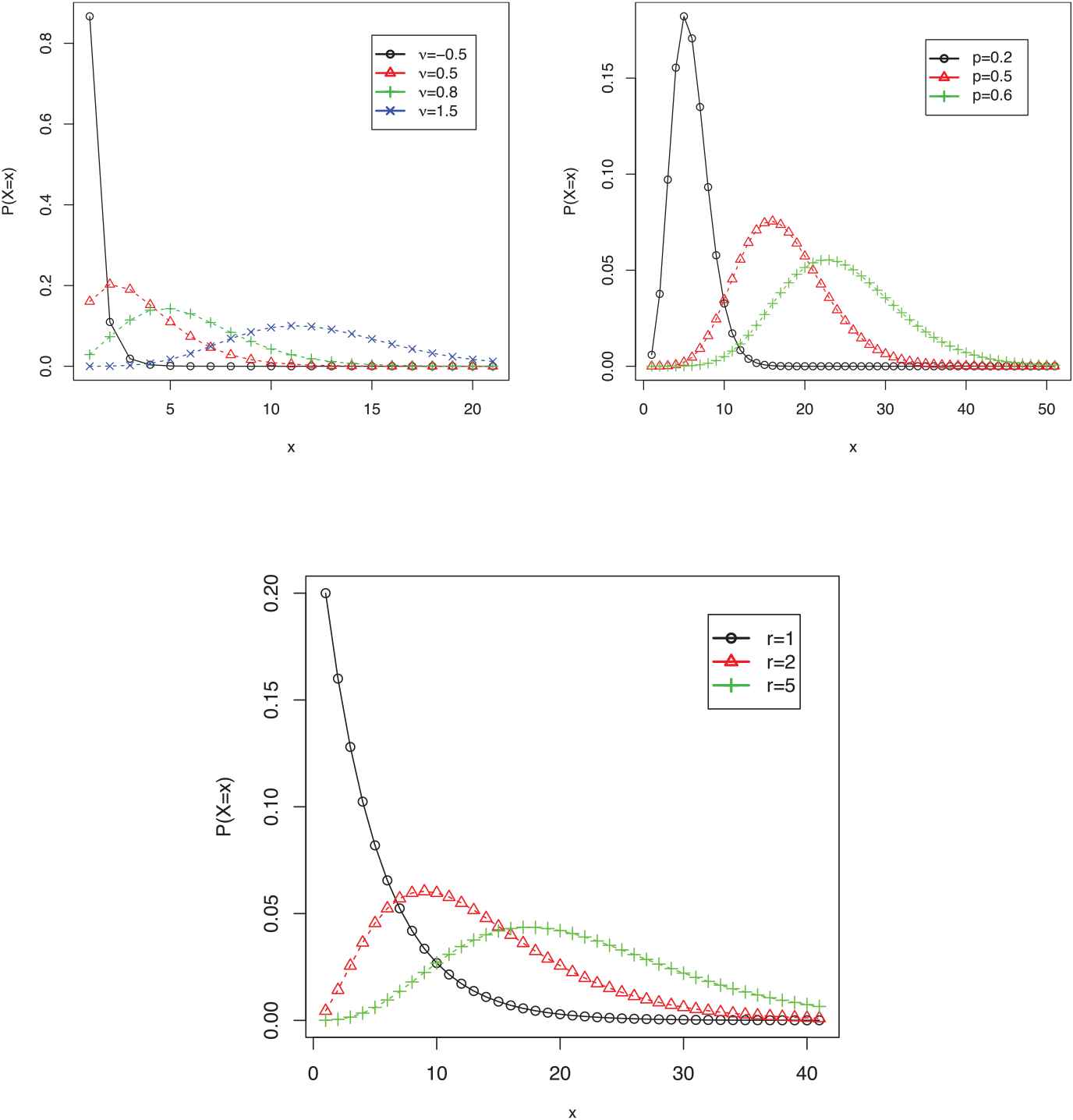
Probability mass function. Left figure: r = 10, p = 0.4. Right figure: r = 10, v = 1.5. Down figure: p = 0.8, v = 2
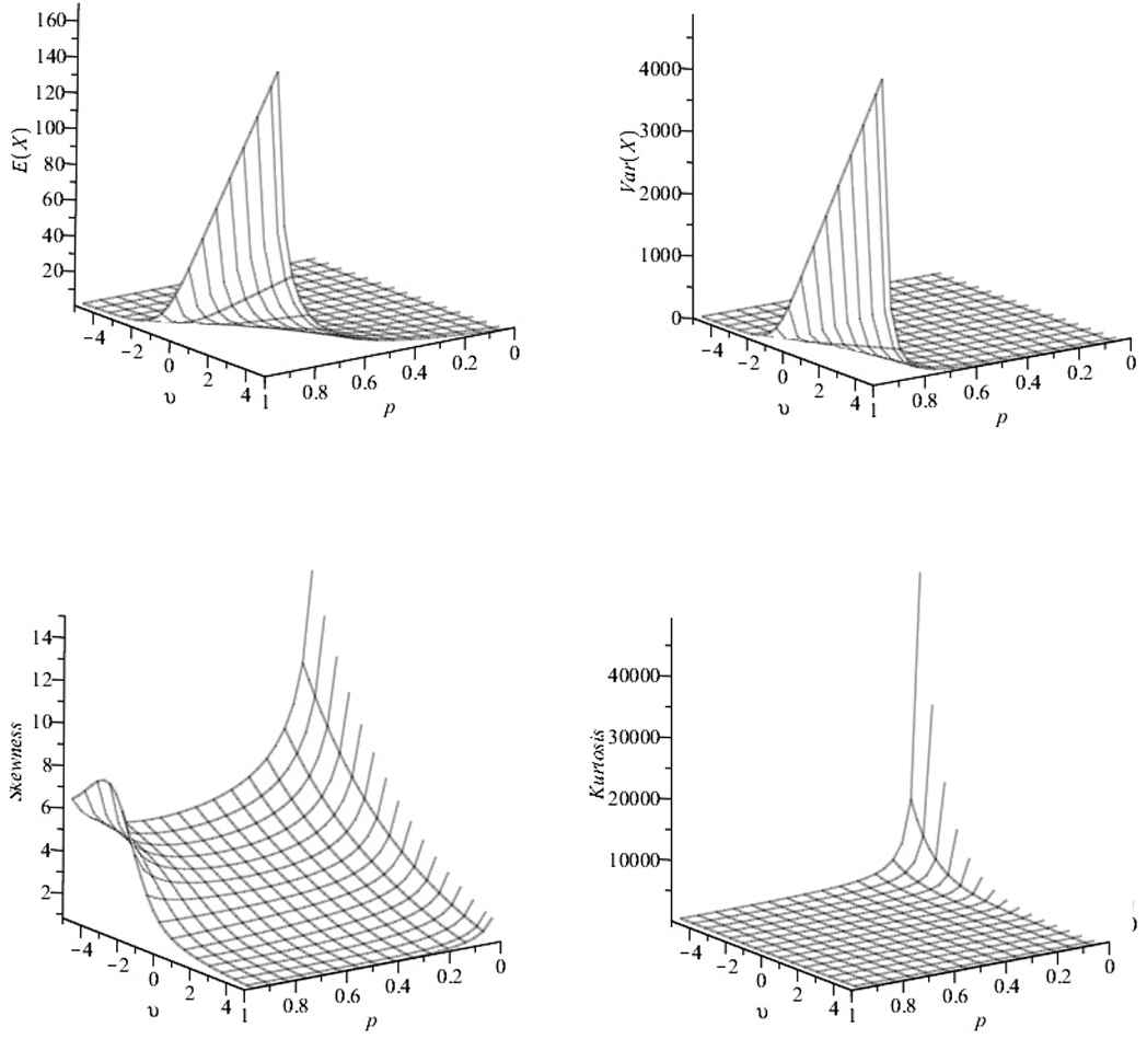
Surface of expectation, variance, skewness and kurtosis of modified negative binomial (Mod-NB) probability mass function with respect to parameter (v and p) while r = 2.
The Mod-NB distribution can be interpreted as a sum of non-independent geometric variables
If we set
It follows from (2) that the Mod-NB distribution belongs to the exponential family on
The probability generating function of this weighted geometric variable is given by
The moment generating function of
3. MAXIMUM LIKELIHOOD ESTIMATION OF THE PARAMETERS
Let
It is of interest to note that
The log-likelihood function for the Mod-NB distribution model based on the observed sample
We can show that
As mentioned earlier since Mod-NB belongs to the exponential distributions family therefore the likelihood equations, based on the observed sample
Since these equations cannot be solved analytically, an iterative method such as the Newton-Raphson method can be used (see Gelman et al. [16], pages 272–273). In each iteration, the expectations, variance and covariance
Notice that the maximum likelihood estimators of the parameters can also be obtained by direct maximization of the log-likelihood function in (4) by using the SAS (PROC NLMIXED) or MaxBFGS routine of the Ox program (Doornik [17]) or optim routine of the R package (R Development Core Team [18]).
4. OVERDISPERSION AND UNDERDISPERSION IN WEIGHTED GEOMETRIC DISTRIBUTION
In this section, we discuss connection between weighted geometric distribution and its overdispersion and underdispersion. We generalize the Mod-NB distribution to the general weight
Theorem 4.1.
Let X be a geometric random variable with mean
Proof.
Let
For fixed
Next, the characteristic variance
Hence, the theorem is proved.
The following corollary is a direct consequence of Theorem 4.1 which enable us to compare weighted geometric distributions in terms of overdispersion and underdispersion.
Corollary 4.1.
Let
If
If
Corollary 4.1 will be clearly useful in cases when
It is of interest to use a statistical test for detecting the overdispersion or underdispersion in observed count data, (Mizère et al. [20]), and it is therefore useful to have a family of count distributions possessing both overdispersion and underdispersion properties with respect to the parameters. In this case, the parameter estimation would lead to an appropriate model within the family for overdispersed or underdispersed count data.
5. REAL DATA EXAMPLE
To illustrate the usefulness and flexibility of the Mod-NB distribution, we consider a real data set. Jaggia and Thosar (1993) model the number of bids received by 126 U.S. firms that were targets of tender offers during the period from 1978 through 1985 and were actually taken over within 52 weeks of the initial offer. The count variable is the number of bids after the initial bid (NUMBIDS) received by the target firm (See Table 1). Here, we have
| Count | 0 | 1 | 2 | 3 | 4 | 5 | 6 | 7 | 8 | 9 | 10 |
| Frequency | 9 | 63 | 31 | 12 | 6 | 1 | 2 | 1 | 0 | 0 | 1 |
| Relative frequency | .071 | .500 | .246 | .095 | .048 | .008 | .016 | .008 | .000 | .000 | .008 |
Takeover bids: Actual frequency distribution.
The form of probability mass functions of BNB and COMP that be used in Table 2, respectively, as follows:
| Number of Takeover Bids | Observed Frequency | Expected Frequency | ||||
|---|---|---|---|---|---|---|
| Mod-NB | NB | B | BNB | COMP | ||
| 0 | 9 | 9.91 | 23.92 | 18.67 | 23.30 | 23.82 |
| 1 | 63 | 61.55 | 38.02 | 39.28 | 37.48 | 36.82 |
| 2 | 31 | 30.78 | 31.84 | 37.19 | 32.45 | 32.45 |
| 3 | 12 | 13.76 | 18.69 | 20.86 | 19.53 | 19.78 |
| 4 | 6 | 5.88 | 8.62 | 7.68 | 8.92 | 8.97 |
| 5 | 1 | 2.45 | 3.33 | 1.94 | 3.19 | 3.12 |
| 6 | 2 | 1.00 | 1.12 | 0.34 | 0.90 | 0.84 |
| 7 | 1 | 0.41 | 0.34 | 0.04 | 0.19 | 0.17 |
| 8 | 0 | 0.16 | 0.09 | 0.00 | 0.03 | 0.03 |
| 9 | 0 | 0.07 | 0.02 | 0.00 | 0.00 | 0.00 |
| 10 | 1 | 0.03 | 0.01 | 0.00 | 0.00 | 0.00 |
| Parameter | – | |||||
| Estimates | – | – | ||||
| – | – | – | – | – | ||
| Kernel of the log-likelihood | −180.1697 | −184.5131 | −201.1203 | −208.3501 | −205.4349 | −206.4554 |
| Chi-square | – | 3.0104 | 29.7659 | 29.3274 | 31.0962 | 33.0807 |
| P-value | – | 0.9812 | 0.0009 | 0.0011 | 0.0005 | 0.0002 |
Mod-NB, modified negative binomial; NB, negative binomial; B, binomial; BNB, beta negative binomial; COMP, COM Poisson binomial.
The goodness of fit of the Mod-NB, NB, B, BNB and COMP distributions for real data.
Suppose
In Table 2, it used the Chi-square statistics for testing the goodness of fit of model on real data. By
6. CONCLUDING REMARKS
We study and discuss here the mathematical properties of the Mod-NB distribution as a extension of the negative binomial distribution. The main advantage of this model is its flexibility to handle overdispersion or underdispersion commonly encountered in count datasets. The Mod-NB distribution is appealing from a theoretical point of view since it belongs to the exponential family as well as to the weighted negative binomial distributions family. Various statistical and probabilistic properties were derived such as moments, probability and moment generating functions and maximum likelihood estimation of parameters. Since the Mod-NB distribution belongs to exponential family, it will also be possible to develop a subjective or objective Bayesian analysis for this model. Work in this direction is currently under progress and we hope to report these findings in a future paper.
AUTHORS' CONTRIBUTIONS
The authors thank the Associate Editor and anonymous reviewers for their useful comments and suggestions on an earlier version of this manuscript which led to this improved one.
Funding Statement
This work has been conducted by University of Zabol, Grant Number: UOZ-GR-9618-14.
REFERENCES
Cite this article
TY  - JOUR
AU  - Ghobad Barmalzan
AU  - Hadi Saboori
AU  - Sajad Kosari
PY  - 2019
DA  - 2019/11/28
TI  - A Modified Negative Binomial Distribution: Properties, Overdispersion and Underdispersion
JO  - Journal of Statistical Theory and Applications
SP  - 343
EP  - 350
VL  - 18
IS  - 4
SN  - 2214-1766
UR  - https://doi.org/10.2991/jsta.d.191105.001
DO  - 10.2991/jsta.d.191105.001
ID  - Barmalzan2019
ER  -