
The Generalized Kumaraswamy-G Family of Distributions
- DOI
- 10.2991/jsta.d.191030.001How to use a DOI?
- Keywords
- Kumaraswamy-G Family; Maximum Likelihood; Order Statistics; Regression
- Abstract
We propose a new class of continuous distributions called the generalized Kumaraswamy-G family which extends the Kumaraswamy-G family defined by Cordeiro and de Castro [1]. Some special models of the new family are provided. Some of its mathematical properties including explicit expressions for the ordinary and incomplete moments, generating function, Rényi entropy, order statistics and characterizations are derived. The new location-scale regression model is introduced based on the new generated distribution. The maximum likelihood is used for estimating the model parameters. The flexibility of the generated family is illustrated by means of two applications to real data sets.
- Copyright
- © 2019 The Authors. Published by Atlantis Press SARL.
- Open Access
- This is an open access article distributed under the CC BY-NC 4.0 license (http://creativecommons.org/licenses/by-nc/4.0/).
1. INTRODUCTION
Recently, the interest in developing more flexible generators remains strong. Many generalized distributions have been developed over the past decades for modeling data in several areas such as biological studies, environmental sciences, economics, engineering, finance and medical sciences. There has been an increased interest in defining new generated families of univariate distributions by introducing additional shape parameters to the baseline model. For example, the Marshall-Olkin-
The generated distributions have attracted several statisticians to develop new models because the computational and analytical facilities available in most symbolic computation software platforms. Several mathematical properties of the extended distributions may be easily explored using mixture forms of exponentiated-G (exp-
Consider a baseline cumulative distribution function (cdf)
In this paper, we define and study a new family of distributions by adding one extra shape parameter in (1) to provide more flexibility to the generated family. To this end, we construct a new generator so-called the generalized Kumaraswamy-G (GK-
The cdf of the GK-
The corresponding pdf of (3) is given by
Henceforth, a random variable
The hazard rate function (hrf) of
Some special cases of the new family are listed in Table 1.
| Reduced Model | Authors | |||
|---|---|---|---|---|
| K- |
Cordeiro and de Castro [1] | |||
| Ex- |
New | |||
| exp- |
Gupta et al. [7] | |||
| – |
Sub-models of the GK-
The rest of the paper is outlined as follows. In Section 2, three special models of GK-G family including Weibull, log-logistic and gamma are presented. In Section 3, some of mathematical properties of the proposed family including linear representation, ordinary and incomplete moments, mean deviations, moment generating function (mgf), Rényi entropy and order statistics are obtained. Maximum likelihood estimation of the model parameters is investigated in Section 4. In Section 5, we provide a simulation study to evaluate the performance of the maximum likelihood method in estimating the parameters of the GK-G family. The log-generalized Kumaraswamy-Weibull regression model is defined in Section 6. Section 7 is devoted to applications to prove empirically the flexibility of the proposed models. Finally, some concluding remarks are given in Section 8.
2. SPECIAL MODELS
In this section, we provide four special models of the GK-
2.1. The GK-Weibull (GKW) Distribution
The Weibull (W) distribution, with positive parameters
The GKW distribution reduces to the GK-exponential (GKE) distribution when
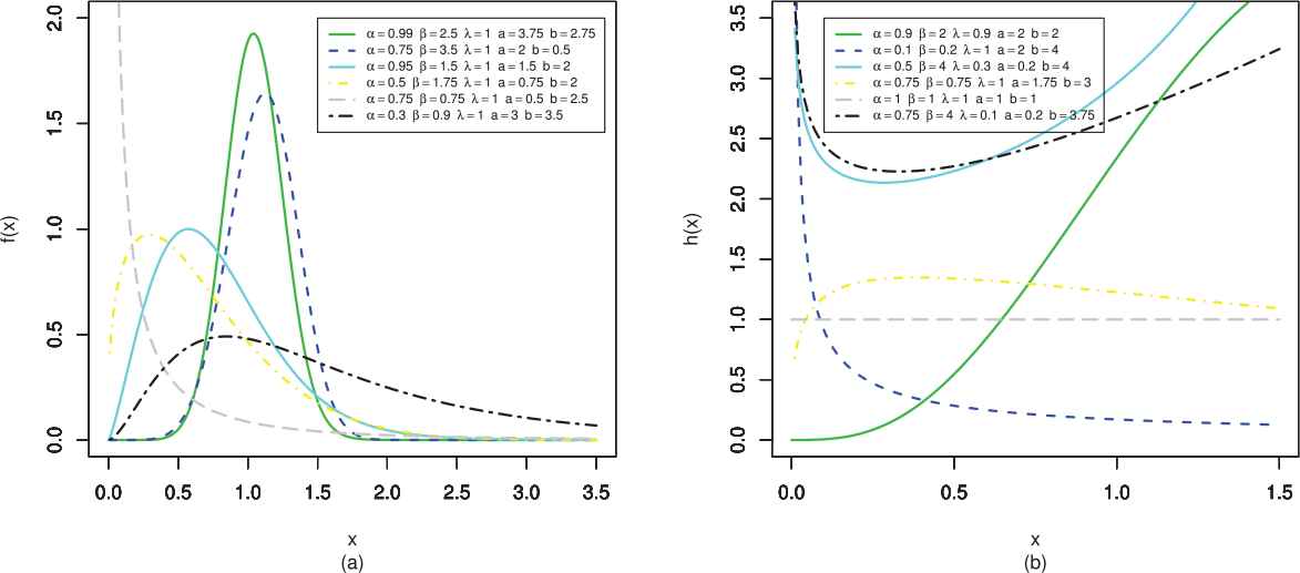
pdf (left) and hrf (right) plots of GK-Weibull (GKW) distribution.
2.2. The GK-Log Logistic (GKLL) Distribution
The log-logistic (LL) distribution with positive parameters
The GKLL model reduces to the LL distribution when
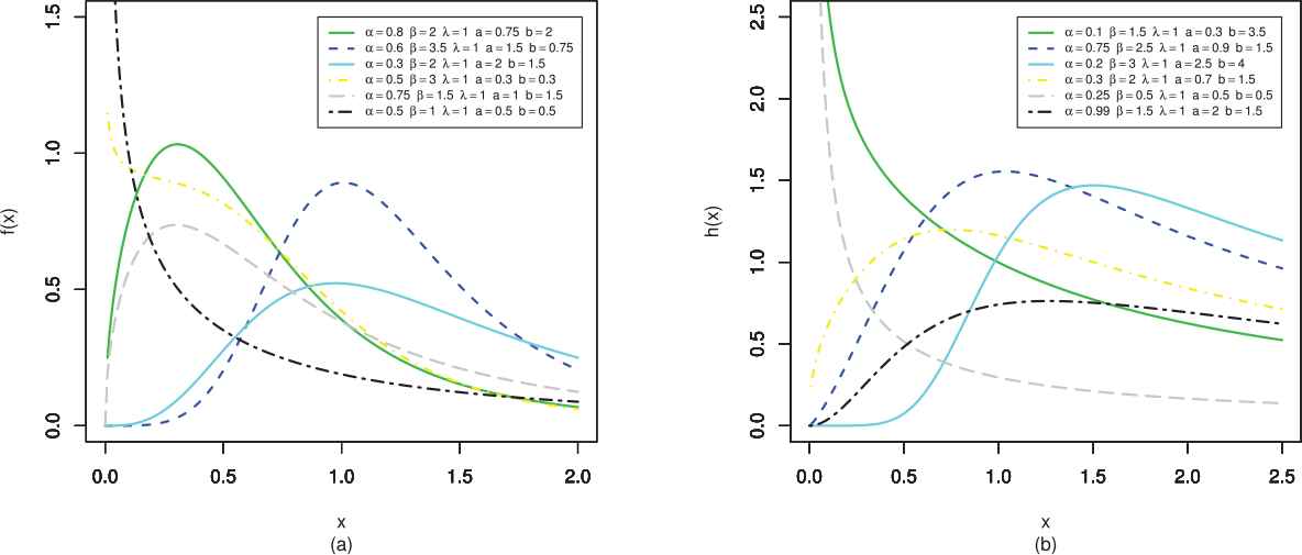
pdf (left) and hrf (right) plots of GK-log logistic (GKLL) distribution.
2.3. The GK-Gamma (GKGa) Distribution
By taking
This distribution reduces to the Ga distribution if
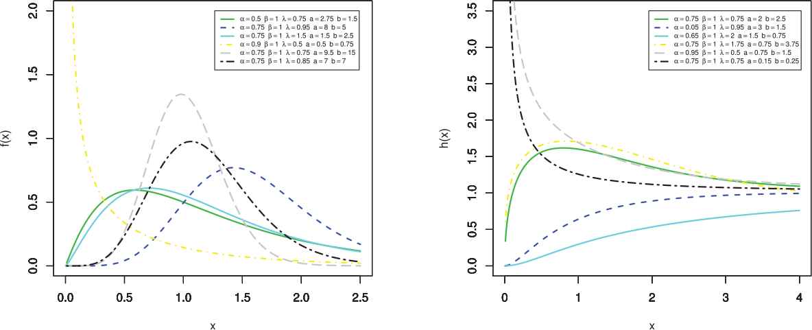
pdf (left) and hrf (right) plots of GK-gamma (GKGa) distribution.
3. MATHEMATICAL PROPERTIES
3.1. Linear Representation
In this section, we provide a useful representation for the GK-
After applying the power series (5) to (4), we obtain
Further, we can write the last equation as
Thus, several mathematical properties of the GK-
The cdf of the GK-
The formulae derived throughout the paper can be easily handled in most symbolic computation software platforms such as Maple, Mathematica and Matlab because of their ability to deal with analytic expressions of formidable size and complexity. Established explicit expressions to evaluate statistical measures can be more efficient than computing them directly by numerical integration. We have noted that the infinity limit in these sums can be substituted by a large positive integer such as 50 for most practical purposes.
3.2. Quantile Function
The quantile function (qf) of
3.3. Moments
Hereafter,
3.4. Generating Function
Here, we provide two formulae for the mgf
A second formula for
3.5. Incomplete Moments
The
The mean deviations about the mean
Now, we provide two ways to determine
A second general formula for
These equations for
3.6. Entropies
The Rényi entropy of a random variable
Using the pdf (4), we can write
Applying the power series (5) to the last term, we obtain
Then, the Rényi entropy of the GK-
3.7. Order Statistics
Order statistics make their appearance in many areas of statistical theory and practice. Let
Using (4) and the above equation, we can write
After a power series expansion, the last equation reduces to
Then, we have
Substituting (10) in (8), the pdf of
(10) reveals that the density function of the GK-
For example, the
4. CHARACTERIZATIONS
Here, we provide two characterization theorems. We will use the following two Lemmas to prove our main results.
Assumptin A.
Suppose the random variable
Lemma 1.
Suppose
Lemma 2.
Suppose
Theorem 1.
Suppose that
Proof.
It is easy to show that if
We prove here the only if condition.
Suppose that
We have
Thus by Lemma 1
On integrating both sides of the above equation, we obtain
Using the boundary condition
Theorem 2.
Suppose that
Proof.
The if condition is easy to show. We will prove here the only if condition.
If
Then
Thus
By Lemma 2, we have
On integrating both sides of the above equation, we obtain
Using the boundary ondition
Remark 1.
5. MAXIMUM LIKELIHOOD ESTIMATION
In this section, we determine the MLEs of the parameters of the new GK-
(12) can be maximized either directly by using the R (optim function), SAS (PROC NLMIXED) or Ox program (sub-routine MaxBFGS) or by solving the nonlinear likelihood equations obtained by differentiating (12).
The score vector components, say
Setting the nonlinear system of equations
6. SIMULATION STUDY
In this subsection, a simulation study is conducted to examine the performance of the MLEs of the generalized Kumaraswamy normal (GKN) parameters. We generate 10,000 samples of size, n = 50, 500 and 1,000 of the GKN model. The precision of the MLEs is discussed by means of the following measures: mean, mean square error (MSE), estimated average length (AL) and coverage probability (CP). The empirical study was conducted with software R. The empirical results are given in Table 2. The values in Table 1 indicate that the estimates are quite stable and, more importantly, are close to the true values for the these sample sizes. The simulation study shows that the maximum likelihood method is appropriate for estimating the GKN parameters. In fact, the means of the parameters tend to be closer to the true parameter values when n increases. This fact supports that the asymptotic normal distribution provides an adequate approximation to the finite sample distribution of the MLEs.
| Mean |
MSE |
||||||||||||||
|---|---|---|---|---|---|---|---|---|---|---|---|---|---|---|---|
| 0.5 | 0.5 | 2 | 0 | 1 | 50 | 0.3641 | 0.6933 | 2.2054 | −0.1111 | 1.0367 | 0.1296 | 0.3960 | 0.2200 | 0.3944 | 0.0857 |
| 500 | 0.3991 | 0.5997 | 2.0905 | −0.0906 | 1.0334 | 0.0814 | 0.1150 | 0.0610 | 0.1732 | 0.0408 | |||||
| 1000 | 0.4669 | 0.5507 | 2.0448 | −0.0245 | 1.0224 | 0.0510 | 0.0547 | 0.0286 | 0.0811 | 0.0205 | |||||
| 0.3 | 2 | 0.5 | 0 | 1 | 50 | 0.0517 | 2.2070 | 0.1416 | −0.0938 | 0.9765 | 1.0513 | 0.8443 | 0.4594 | 0.0919 | 0.0258 |
| 500 | 0.2085 | 2.1592 | 0.3098 | −0.0988 | 0.9879 | 0.4034 | 0.3933 | 0.1505 | 0.0471 | 0.0118 | |||||
| 1000 | 0.1871 | 2.1492 | 0.3888 | −0.0642 | 0.9919 | 0.3583 | 0.3828 | 0.0755 | 0.0612 | 0.0089 | |||||
| 0.7 | 1.5 | 2.5 | 0 | 1 | 50 | 0.4229 | 2.0211 | 2.8649 | −0.2270 | 1.1292 | 0.2230 | 0.8115 | 0.3188 | 0.3174 | 0.1674 |
| 500 | 0.5629 | 1.8111 | 2.6869 | −0.1810 | 1.0252 | 0.0730 | 0.4305 | 0.1898 | 0.1404 | 0.0165 | |||||
| 1000 | 0.6727 | 1.5157 | 2.4998 | −0.0182 | 0.9933 | 0.0294 | 0.0253 | 0.0144 | 0.0108 | 0.0084 | |||||
Simulation results of the GK-N distribution for several values of parameters.
7. THE LOG-GENERALIZED KUMARASWAMY-WEIBULL (LGKW) REGRESSION MODEL
The GKW distribution with five parameters,
The corresponding survival function is
Parametric regression models to estimate univariate survival functions for censored data are widely used. A parametric model that provides a good fit to lifetime data tends to yield more precise estimates of the quantities of interest. Based on the LGKW density, we propose a linear location-scale regression model linking the response variable
Consider a sample
Further, we can use the likelihood ratio (LR) statistic for comparing LGKW model with its sub-models. We consider the partition
8. APPLICATIONS
8.1. First Application
In this section, we illustrate the fitting performance of GKGa distribution by means of real data sets. We compare the fitting performance of GKGa distribution with its sub-models. The sub-models of the GKGa distribution are given as follows: (i) Gamma distribution, (ii) exponentiated Gamma distribution, (iii) extended Gamma distribution (new), (iv) Kumaraswamy-Gamma distribution.
The used data set consists of prices (
| Data set | Mean | Median | SD | ||
|---|---|---|---|---|---|
| Prices ( |
3.3 | 2.7 | 1.9 | 2.8 | 16.7 |
Descriptive statistics of turbocharger failure time data set (
The measures of goodness-of-fit including the–log-likelihood function evaluated at the MLEs, Anderson-Darling (
Table 4 gives the parameter estimates and their corresponding errors, the
| Models | |||||||||
|---|---|---|---|---|---|---|---|---|---|
| Ga | 1 | 1 | 1 | 4.071 | 1.242 | 4.308 | 0.646 | 777.719 | 0.035 |
| − | − | − | 0.267 | 0.086 | |||||
| Ex-Ga | 0.005 | 1 | 681.384 | 4.247 | 0.848 | 1.668 | 0.234 | 758.5601 | 0.422 |
| 0.011 | − | 93.441 | 0.294 | 0.115 | |||||
| Exp-Ga | 1 | 111.785 | 1 | 0.078 | 0.602 | 1.175 | 0.156 | 754.536 | 0.550 |
| − | 44.434 | − | 0.030 | 0.033 | |||||
| K-Ga | 1 | 2.500 | 0.344 | 3.426 | 2.310 | 1.558 | 0.215 | 757.241 | 0.244 |
| − | 0.011 | 0.017 | 0.005 | 0.005 | |||||
| GKGa | 0.005 | 449.042 | 437.736 | 0.016 | 0.404 | 0.433 | 0.047 | 748.677 | 0.916 |
| 0.024 | 94.829 | 44.201 | 0.040 | 0.063 |
Parameters estimates of proposed model and other competitive models.
| Models | Hypotheses | LR Statistic w | p Value |
|---|---|---|---|
| GKGa vs Ga | 58.084 | ||
| GKGa vs Ex-Ga | 19.766 | ||
| GKGa vs Exp-Ga | 11.718 | ||
| GKGa vs K-Ga | 17.128 |
LR tests results for first data set.
Based on Table 5, we reject all the null hypotheses and conclude that the GKGa fits the used data set better than the its sub-models according to the LR test.
We also plotted the fitted pdfs of the considered models for the sake of visual comparison, in Figure 4. Figure 4(a) represents that the GKGa fits the right skewed data very well. In addition, we presented the plots of the fitted density, cumulative and survival functions as well as the probability-probability (P-P) plot for the GKGa model in Figure 4(b). These plots reveal that the GKGa distribution is a suitable model for the data.
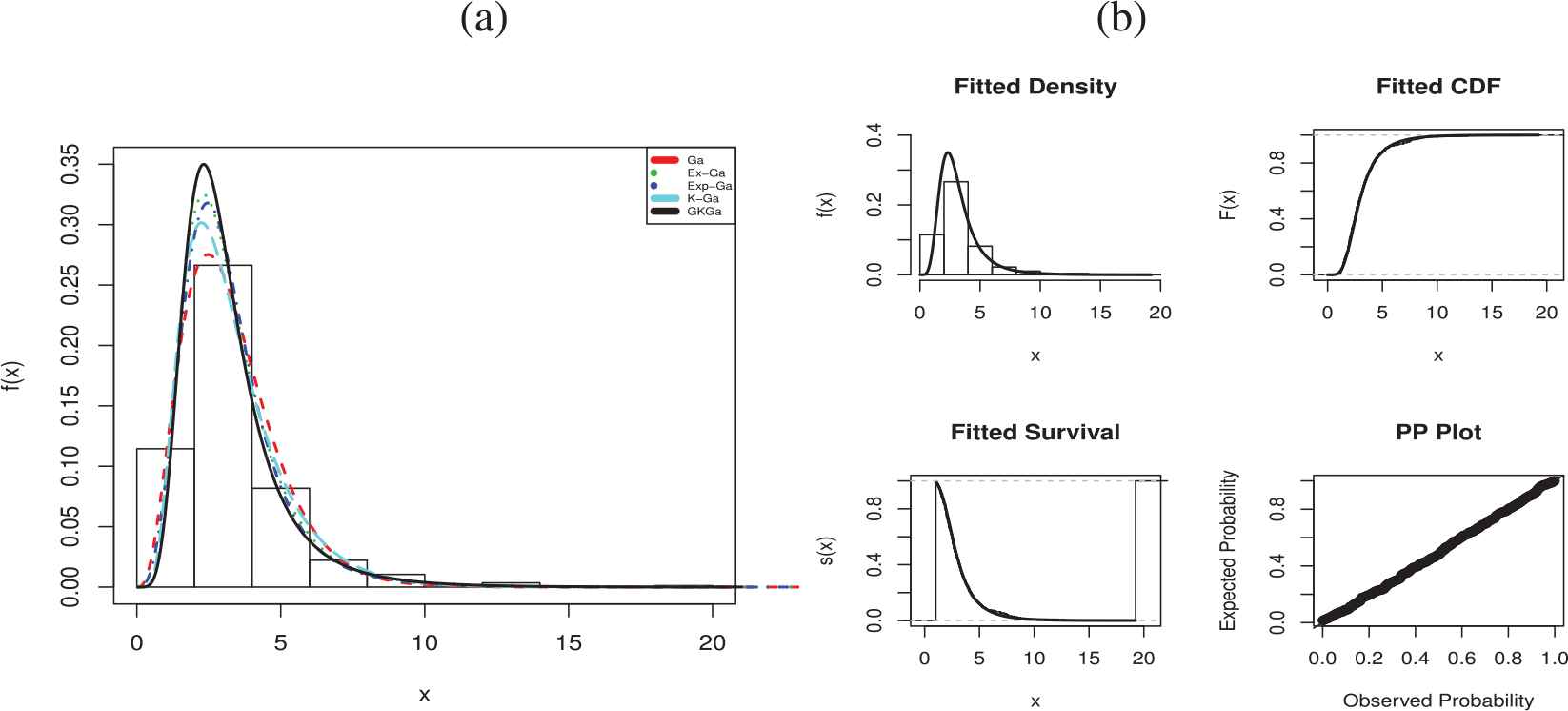
(a) Fitted densities of models and (b) fitted functions of GK-gamma (GKGa) for used data set.
8.2. Second Application
The dataset contains 100 observations on HIV+ subjects belonging to an Health Maintenance Organization(HMO). The HMO wants to evaluate the survival time of these subjects. In this hypothetical data set, subjects were enrolled from January 1, 1989 until December 31, 1991. Study follow-up then ended on December 31, 1995. This data set are reported in Hosmer and Lemeshow [9] and also can be found in R package Bolstad2. The variables involved in the study are:
The aim of the study is to relate the survival time (
| Model | ||||||||
|---|---|---|---|---|---|---|---|---|
| LW | 1 | 1 | 1 | 1.070 | 3.003 | −1.051 | 146.437 | 298.875 |
| − | − | − | (0.088) | (0.166) | (0.239) | |||
| [ |
[ |
|||||||
| LGKW | 4.07E-09 | 22.383 | 25.742 | 3.675 | −2.255 | −0.865 | 140.904 | 293.808 |
| (0.0001) | (4.098) | (4.379) | (1.917) | (4.393) | (0.271) | |||
| [0.607] | [0.001] |
MLEs of the parameters (standard errors in parentheses and
A comparison of the LGKW regression model with LW regression model using LR statistics is performed. LR test statistic is calculated as 11.066 and corresponding p-value is 0.011. These results indicate that the LGKW model provides better fit to these data than the LW regression model.
The plots in Figure 5(a) provide the Kaplan-Meier (KM) estimate and the estimated survival functions of the LGKW regression model. There is significant difference between drug users and drug non-users survival functions. The plots of the hrf in Figure 5(b) corresponding to the survival time variable under the LGKW regression model indicate that the hrf is larger for drug non-users than drug users. Based on these plots, we conclude that the LGKW regression model provides a good fit to these data.
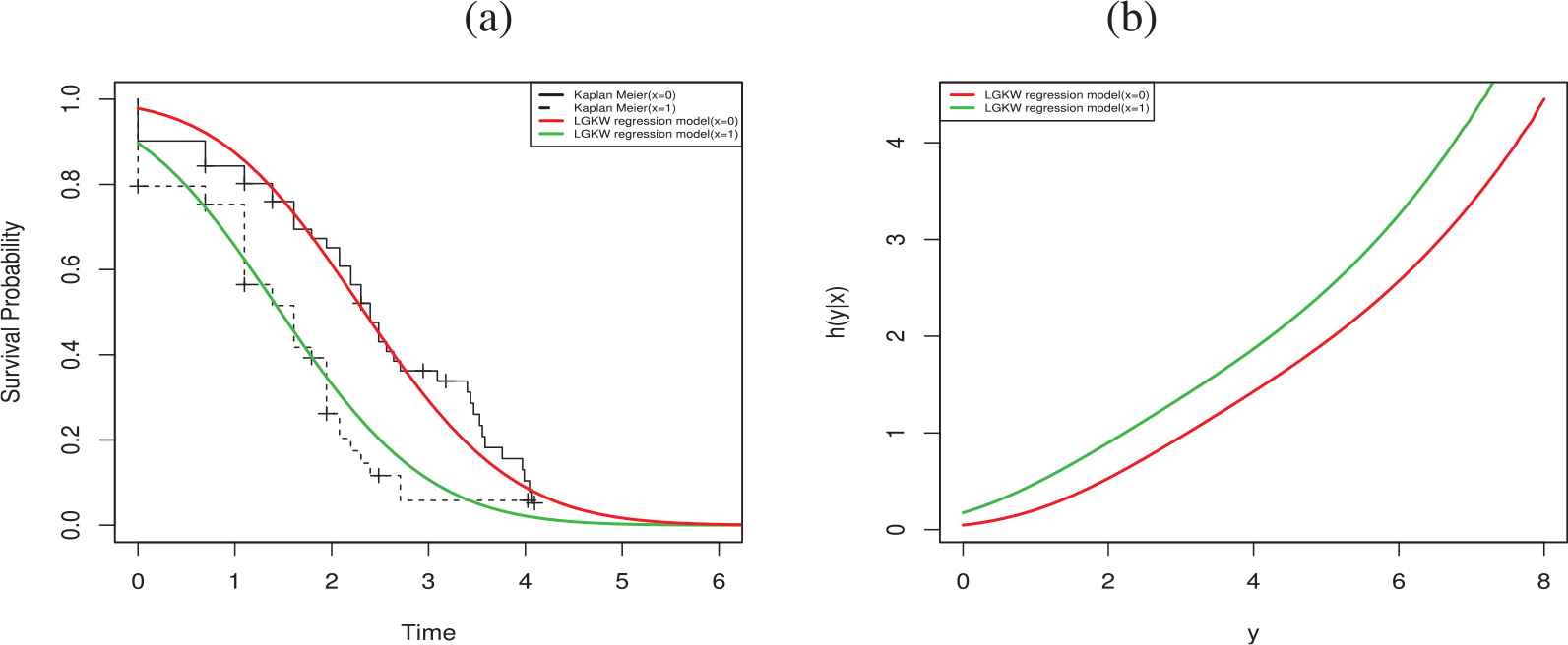
(a) Estimated survival functions and the empirical survival: :Log-generalized Kumaraswamy-Weibull (LGKW) regression model versus KM. (b) Fitted hrf using the LGKW regression model for the history of drug use.
9. CONCLUSION
We propose a new class of continuous distributions named the generalized Kumaraswamy family to extended the some classes of distributions such as Exp-G by Gupta et al. [7] and K-G by Cordeiro and de Castro [1]. We obtain some mathematical properties of proposed family including quantile function, moments, generating function, entropies, order statistics and probability weighted moments. The maximum likelihood method is used to estimate the model parameters and the performance of the maximum likelihood estimators are discussed in terms of biases, mean squared errors, coverage probability and estimated average length by means of Monte-Carlo simulation study. The usefulness of the proposed family is discussed by means of two real data applications.
CONFLICT OF INTEREST
The authors declare no conflict of interest.
AUTHORS' CONTRIBUTIONS
All authors contributed equally to this work.
Funding Statement
This work has no fund.
ACKNOWLEDGMENTS
The authors would like to thank the Editor in Chief and two reviewers for their constructive comments which improved the final version of the paper.
REFERENCES
Cite this article
TY  - JOUR
AU  - Zohdy M. Nofal
AU  - Emrah Altun
AU  - Ahmed Z. Afify
AU  - M. Ahsanullah
PY  - 2019
DA  - 2019/11/20
TI  - The Generalized Kumaraswamy-G Family of Distributions
JO  - Journal of Statistical Theory and Applications
SP  - 329
EP  - 342
VL  - 18
IS  - 4
SN  - 2214-1766
UR  - https://doi.org/10.2991/jsta.d.191030.001
DO  - 10.2991/jsta.d.191030.001
ID  - Nofal2019
ER  -