
On a Generalized Burr Life-Testing Model: Characterization, Reliability, Simulation, and Akaike Information Criterion
- DOI
- 10.2991/jsta.d.190818.001How to use a DOI?
- Keywords
- Akaike information criterion; Characterization; Reliability; Truncated moment
- Abstract
For a continuous random variable X, M. Shakil, B.M.G. Kibria, J. Stat. Theory Appl. 9 (2010), 255–282, introduced a generalized Burr increasing, decreasing, and upside-down bathtub failure rate life-testing model. In this paper, we provide some characterizations of this life-testing model by truncated first moment, order statistics and upper record values. We also investigate the reliability, simulation, and Akaike information criterion for this model.
- Copyright
- © 2019 The Authors. Published by Atlantis Press SARL.
- Open Access
- This is an open access article distributed under the CC BY-NC 4.0 license (http://creativecommons.org/licenses/by-nc/4.0/).
1. INTRODUCTION
For a continuous positive random variable X, the following increasing, decreasing, and upside-down bathtub failure rate life testing five-parameter family of continuous probability density function (pdf) in terms of beta function has been introduced by Shakil and Kibria [1]:
The
The first moment, when
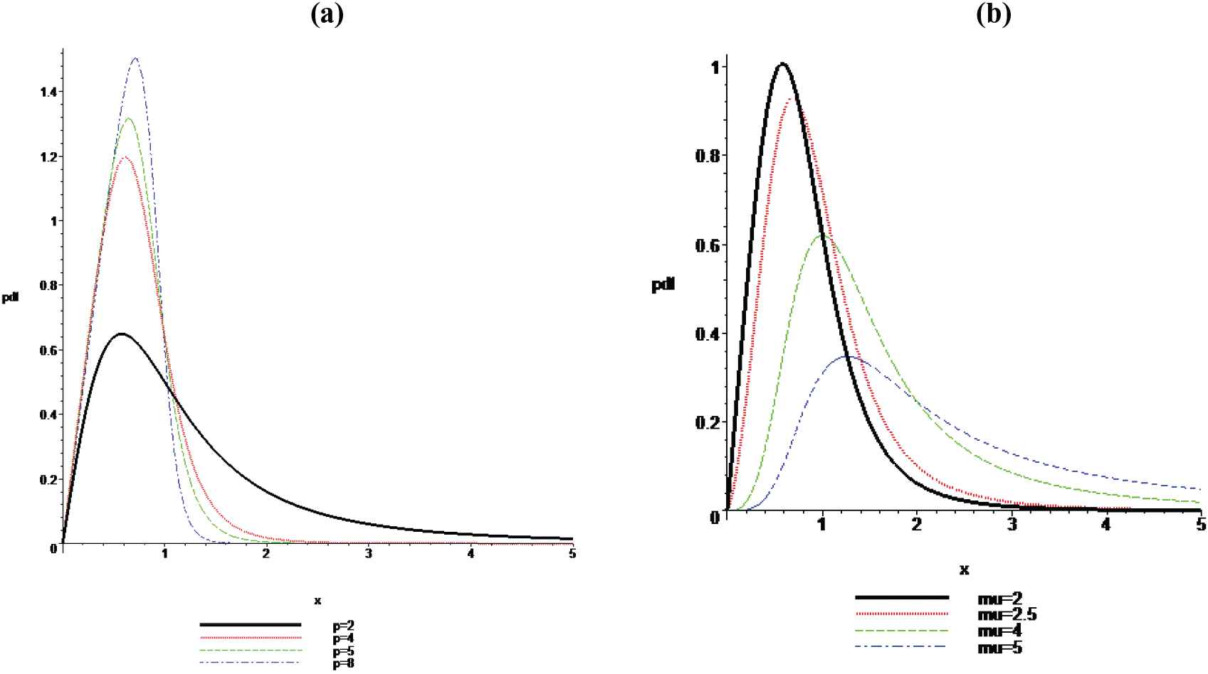
PDF Plots for: (a) α = 1, β = 1, v = 2, μ = 2, p = 2, 4, 5, 8 (left); and (b) α = 1, β = 1, v = 2, p = 3, μ = 2, 2.5, 4, 5 (right).
The effects of the parameters can easily be seen from the above graphs. From these graphs, it is observed that the above-said distribution is right skewed. Also, since the mode is the value of
The paper is organized as follows. In Section 2, we present some characterization results. We provide reliability results in Section 3. The Akaike information criterion (AIC), etc., are discussed in Section 4. Finally, some concluding remarks are presented in Section 5.
2. CHARACTERIZATION RESULTS
Since the truncated distributions arise in practical statistics where the ability of record observations is limited to a given threshold or within a specified range, there has been a great interest, in recent years, in the characterizations of probability distributions by truncated moments. The development of the general theory of the characterizations of probability distributions by truncated moment began with the work of Galambos and Kotz [2], Kotz and Shanbhag [3], Glänzel et al. [4], and Glänzel [5]. For recent developments, we refer our readers to Ahsanullah [6], and references therein. In this section, we provide the proposed characterizations of the said distribution by truncated moment, order statistics, and upper record values. For this, we shall need the following assumption and lemmas.
2.1. Assumption and Lemmas
Assumption 2.1.1.
Suppose the random variable
Lemma 2.1.1.
Under the Assumption 2.1.1, if
Proof:
See Ahsanullah and Shakil [7].
Lemma 2.1.2.
Under the Assumption 2.1.1, if
Proof.
See Ahsanullah and Shakil [7].
2.2. Characterization by Truncated First Moment
We provide the proposed characterizations in Theorems 2.2.1 and 2.2.2.
Theorem 2.2.1.
If the random variable
Proof.
Suppose that
Conversely, suppose that
Then, differentiating
Since, by Lemma 2.1.1, we have
On integrating the above expression with respect to
Theorem 2.2.2.
If the random variable
Proof.
The proof is omitted, since it is similar to the Theorem 2.2.1, and easily follows from Lemma 2.1.2.
2.3. Characterization by Order Statistics
Suppose that
Now, based on the order statistics, we will provide the characterizations in Theorem 2.3.1 and 2.3.2 below.
Theorem 2.3.1.
Assume that the random variable
Proof.
Since
Theorem 2.3.2
Assume that the random variable
Proof.
Since
2.4. Characterization by Upper Record Values
Suppose that
Theorem 2.4.1.
Assume that the random variable
Proof.
Since
3. RELIABILITY ANALYSIS
The reliability analysis of lifetime distributions plays an important role in modelling many real world phenomena in the fields of biological, economics, engineering, physical, and other pure and applied sciences. For a nonrepairable population, we define the failure rate as the instantaneous rate of failure for the survivors to time t during the next instant of time. We investigate some reliability properties of the said model. The corresponding survival (or reliability) and the hazard (or failure rate) functions of the said model are respectively given by
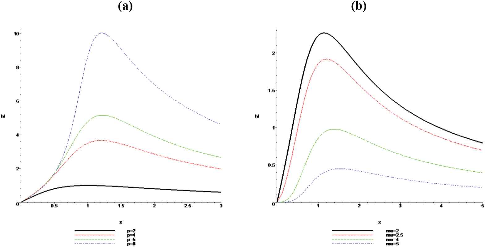
Failure Rate (hf) Plots for (a) α = 1, β = 1, v = 2, μ = 2, p = 2, 4, 5, 8 (left); and (b) α = 1, β = 1, v = 2, p = 3, μ = 2, 2.5, 4, 5 (right).
The effects of the parameters are obvious from these figures. The increasing, then decreasing, and upside-down bathtub shape behaviors of the failure rate function,
4. ESTIMATION, SIMULATION, AND AIC OF THE PERFORMANCE OF GENERALIZED BURR LIFE-TESTING MODEL
4.1. The Method of Moments
From the
4.2. The Method of Maximum Likelihood
Given a sample
4.3. Simulation
In this section, we use simulation to compare the performances of the different methods of estimation mainly with respect to their biases, mean square errors (MSE), and variances for different sample sizes. A numerical study is performed using Mathematica 9 software. Different sample sizes are considered through the experiments at size n = 15, 20, 30, and 50 for different values of the parameters
| n | Par | Init | MLE | Bais | MSE | Init | MLE | Bais | MSE |
|---|---|---|---|---|---|---|---|---|---|
| α | 1.2 | 1.2536 | 0.0535 | 0.0219 | 1.4 | 1.4435 | 0.0435 | 0.0240 | |
| β | 1.2 | 1.1700 | −0.0300 | 0.0195 | 1.4 | 1.3829 | −0.0171 | 0.0252 | |
| 10 | 1.4 | 1.0709 | −0.3291 | 0.1736 | 1.6 | 1.2408 | −0.3593 | 0.3325 | |
| µ | 0.5 | 0.4269 | −0.0731 | 0.0085 | 0.5 | 0.4348 | −0.0652 | 0.0084 | |
| p | 0.8 | 1.5221 | 0.7221 | 0.9093 | 0.7 | 0.8870 | 0.1870 | 0.0993 | |
| α | 1.2 | 1.2437 | 0.0437 | 0.0101 | 1.4 | 1.4271 | 0.0271 | 0.0104 | |
| β | 1.2 | 1.1644 | −0.0356 | 0.0102 | 1.4 | 1.3842 | −0.0158 | 0.0128 | |
| 20 | 1.4 | 1.0480 | −0.3520 | 0.1424 | 1.6 | 1.1871 | −0.4129 | 0.1937 | |
| µ | 0.5 | 0.4240 | −0.0760 | 0.0073 | 0.5 | 0.4344 | −0.0656 | 0.0064 | |
| p | 0.8 | 1.4138 | 0.6138 | 0.5405 | 0.7 | 0.8703 | 0.1703 | 0.0618 | |
| α | 1.2 | 1.2390 | 0.0390 | 0.0069 | 1.4 | 1.4216 | 0.0215 | 0.0069 | |
| β | 1.2 | 1.1649 | −0.0351 | 0.0075 | 1.4 | 1.3854 | −0.0146 | 0.0087 | |
| 30 | 1.4 | 1.0382 | −0.3618 | 0.1413 | 1.6 | 1.1794 | −0.4206 | 0.1932 | |
| µ | 0.5 | 0.4241 | −0.0759 | 0.0068 | 0.5 | 0.4343 | −0.0657 | 0.0057 | |
| p | 0.8 | 1.3944 | 0.5944 | 0.4625 | 0.7 | 0.8622 | 0.1622 | 0.0488 | |
| α | 1.2 | 1.2386 | 0.0385 | 0.0044 | 1.4 | 1.4273 | 0.0273 | 0.0047 | |
| β | 1.2 | 1.1608 | −0.0392 | 0.0049 | 1.4 | 1.3743 | −0.0257 | 0.0057 | |
| 50 | 1.4 | 1.0354 | −0.3646 | 0.1382 | 1.6 | 1.1835 | −0.4165 | 0.1826 | |
| µ | 0.5 | 0.4223 | −0.0777 | 0.0066 | 0.5 | 0.4297 | −0.0703 | 0.0058 | |
| p | 0.8 | 1.3558 | 0.5558 | 0.3626 | 0.7 | 0.8410 | 0.1410 | 0.0331 |
MLE, maximum likelihood estimate; MSE, mean square errors.
The parameter estimation of the generalized burr life-testing model using MLE.
If we review Table 1, it is observed that as the sample size increases, both absolute bias and MSE decrease and converge to close to true values of parameters.
4.4. Akaike Information Criterion
As pointed out by Emiliano et al. [17], the choice of the best model is crucial in modeling data. Akaike [18,19] developed an entropy-based information criterion to test the applicability, relative measures, and performance of lifetime distributions to real life data, known in the literature as the AIC. Later, various information criteria for testing the goodness of fit of lifetime probability models were developed by different authors and researchers, among them the corrected Akaike information criterion (CAIC) (Sugiura [20]), the Bayesian information criterion (BIC) (Schwarz [21]), the generalized information criterion (GIC) (Konishi and Kitagawa [22]), and Hannan–Quinn information criterion (HQIC) (Hannan and Quinn [23]), are notable. For details on these, the interested readers are referred to Emiliano et al. [17], and references therein. In this section, we investigate the performance of the generalized Burr life-testing model by using various criteria such as
Example 1.
This example considers the data for average annual percent change in private health insurance premiums (All Benefits: Health Services and Supplies), Calendar Years 1969–2007 (SOURCE: Centers for Medicare & Medicaid Services, Office of the Actuary, National Health Statistics Group), which are provided in Table 2. Based on this example, we test the goodness of fit of the generalized Burr life-testing model and compare it with the Burr's type XII, log-logistic, gamma, and lognormal distributions.
| 14.4, 14.0, 15.4, 9.4, 11.7, 15.0, 24.9, 20.7, 12.5, 14.9, 12.6, 16.7, 13.8, 11.0, 12.9, 10.1, 1.9, 8.5, 16.5, 15.3, 13.3, 9.8, 8.4, 7.9, 3.7, 5.1, 4.6, 4.4, 5.4, 6.1, 8.0, 10.0, 11.2, 10.1, 6.4, 6.7, 5.7, 5.8 |
Average annual percent change in private health insurance premiums.
The mean, median, skewness, and kurtosis of this data are 10.7, 10.1, 0.603, and 0.557 respectively. We can see that the data is right skewed. The estimators of the unknown parameters of each distribution is obtained by the maximum likelihood method. In order to compare the generalized Burr life-testing model with other models, we use
| Model | MLEs and S. E | ||||
|---|---|---|---|---|---|
| New Model |
|||||
| Burr XII |
- | - | - | ||
| Gamma |
- | - | - | ||
| Log Logistic |
- | - | - | ||
| Log normal |
- | - | - | ||
The MLEs and S.E of the model parameters for data set in Table 2.
The variance covariance matrix
The following Table 4 shows the values of
| Distribution | −2ln L | AIC | BIC | CAIC | HQIC |
|---|---|---|---|---|---|
| New Model | 250.804 | 260.804 | 258.814 | 262.569 | 263.857 |
| Burr XII | 431.625 | 435.625 | 434.829 | 435.949 | 436.846 |
| Gamma | 504.553 | 508.553 | 507.757 | 508.877 | 509.774 |
| Log Logistic | 682.54 | 439.075 | 438.279 | 439.4 | 440.297 |
| Log normal | 473.113 | 477.113 | 476.317 | 477.437 | 478.334 |
AIC, Akaike information criterion; BIC, Bayesian information criterion; CAIC, corrected Akaike information criterion; HQIC, Hannan–Quinn information criterion.
The AIC, BIC, CAIC, and HQIC statistics for the data set in Table 2.
In Fig. 3 below, we provide the plots of estimated densities of the fitted generalized Burr life-testing model, Burr's type XII, log-logistic, gamma and lognormal models for the data set in Table 2.
Estimated densities of the models for data set in Table 2.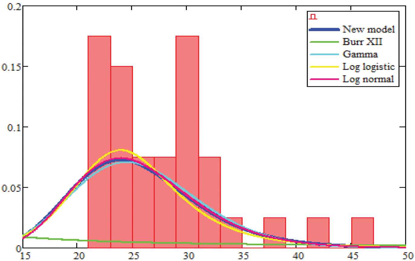
In our above analysis, the Table 3 shows the MLE's of the parameters of the fitted generalized Burr life testing and other distributions to the data set in Table 2. Further, Table 4 shows the values of
5. CONCLUDING REMARKS
Since the truncated distributions arise in practical statistics where the ability of record observations is limited to a given threshold or within a specified range, we investigate, in this paper, some characterizations of the five-parameter continuous life-testing continuous probability distribution of Shakil and Kibria [1] by truncated first moment, order statistics, and upper record values. We also investigate some reliability properties, and Akaike (AIC) and other information criterion to test the measure of the goodness of fit of the said model. It is hoped that the findings of this paper will be quite useful for researchers in the fields of reliability, probability, statistics, and other applied sciences.
CONFLICT OF INTEREST
The authors declare that they have no Conflict of Interests or Competing Interests.
AUTHORS' CONTRIBUTIONS
All the authors have fully contributed to the article, and have read and approved the final manuscript.
Funding Statement
There are no sources of funding for the research.
ACKNOWLEDGMENT
The authors are thankful to the editor-in-chief and the referees for their valuable comments and suggestions, which certainly improved the presentation of the paper.
REFERENCES
Cite this article
TY  - JOUR
AU  - M. Ahsanullah
AU  - M. Shakil
AU  - B. M. Golam Kibria
AU  - M. Elgarhy
PY  - 2019
DA  - 2019/08/30
TI  - On a Generalized Burr Life-Testing Model: Characterization, Reliability, Simulation, and Akaike Information Criterion
JO  - Journal of Statistical Theory and Applications
SP  - 259
EP  - 269
VL  - 18
IS  - 3
SN  - 2214-1766
UR  - https://doi.org/10.2991/jsta.d.190818.001
DO  - 10.2991/jsta.d.190818.001
ID  - Ahsanullah2019
ER  -