
A Multivariate Skew-Normal Mean-Variance Mixture Distribution and Its Application to Environmental Data with Outlying Observations
- DOI
- 10.2991/jsta.d.190617.001How to use a DOI?
- Keywords
- Multivariate distribution; Birnbaum–Saunders; ECM algorithm; Outliers; Mean-variance mixtures
- Abstract
The presence of outliers, skewness, kurtosis, and dependency are well-known challenges while fitting distributions to many data sets. Developing multivariate distributions that can properly accomodate all these aspects has been the aim of several researchers. In this regard, we introduce here a new multivariate skew-normal mean-variance mixture based on Birnbaum–Saunders distribution. The resulting model is a good alternative to some skewed distributions, especially the skew-t model. The proposed model is quite flexible in terms of tail behavior and skewness, and also displays good performance in the presence of outliers. For the determination of maximum likelihood estimates, a computationally efficient Expectation-Conditional-Maximization (ECM) algorithm is developed. The performance of the proposed estimation methodology is illustrated through Monte Carlo simulation studies as well as with some real life examples.
- Copyright
- © 2019 The Authors. Published by Atlantis Press SARL.
- Open Access
- This is an open access article distributed under the CC BY-NC 4.0 license (http://creativecommons.org/licenses/by-nc/4.0/).
1. INTRODUCTION
Although normal distribution has a central role in statistical analysis, the presence of outliers or atypical observations becomes problematic in some applications. This problem often occurs in some fields such as environmental and financial sciences. For example, in a random sample of some variables from water quality or air pollution in a specific area, it is quite common to encounter some outliers in the data. Similarly, outlying observations may be seen in stock returns analysis. For further details on this issue, one may refer to [1] and [2]. When data are noisy, fitting a suitable distribution does become a challenge. Adding a tail or skewness parameter to a normal distribution is a recognized method to accommodate the presence of possible outliers. Two well-known formulations that follow this approach are by Barndorff-Nielsen [3] and Azzalini [4].
Normal mean-variance mixture (NMVM) distributions were introduced by Barndorff-Nielsen [3]. Specifically, if Y be a
A positive random variable
Let the random variable Y be as in (1), where
The other members of NMVM class of distributions can be introduced similarly by choosing other suitable mixing random variable
Now, assuming
To shift from symmetric distributions to asymmetric ones, Azzalini [4] proposed the univariate skew-normal (SN) distribution, which can be used as a substitute for normal distribution in the modeling of data displaying some asymmetry. The multivariate version of SN (MSN) distribution was introduced by Azzalini and Dalla Valle [10] and Arellano-Valle and Genton [11], which extends the multivariate normal model by allowing a shape parameter to account for skewness.
A random vector Y is said to follow a
According to Arellano-Valle and Genton [11], the MSN distribution has a convenient stochastic representation as
If
The aim of this paper is to introduce a multivariate skew-normal mean-variance mixture based on BS (SNMVBS) distribution. The random variable
Tamandi et al. [13] studied the univariate SNMVBS and discussed some of its properties. The modeling of correlated data in the presence of outliers provides a main motivation for extending the univariate SNMVBS to multivariate setup. On the other hand, the SNMVBS distribution serves as an alternative to skew-t (ST) model introduced by Azzalini and Capitanio [14]. The ST distribution is a SN mean-variance mixture distribution, where the mixing distribution is
The rest of this paper proceeds as follows. Section 2 introduces the multivariate SNMVBS distribution and then discusses some of its characteristics. Section 3 develops an ECM algorithm for estimating the parameters of SNMVBS distribution. In Section 4, asymptotic properties of the ML estimators are investigated using simulations. Section 5 illustrates some applications of the SNMVBS distribution in modeling environmental data. Finally, Section 6 provides some concluding remarks.
2. MULTIVARIATE SNMVBS DISTRIBUTION
Let Y be a random variable following the representation in (5), where
Theorem 2.1.
If the random vector Y follows the representation in (6), then the PDF of Y is given by
A detailed proof of this theorem is given in Appendix A. The notations in Theorem 2.1 will be used throughout the paper. Figure 1 displays some examples of the density function in (7). These figures present four different densities and the corresponding contour plots for Density functions and corresponding contours of skew-normal mean-variance mixture based on Birnbaum–Saunders (SNMVBS) distribution. From top to bottom: 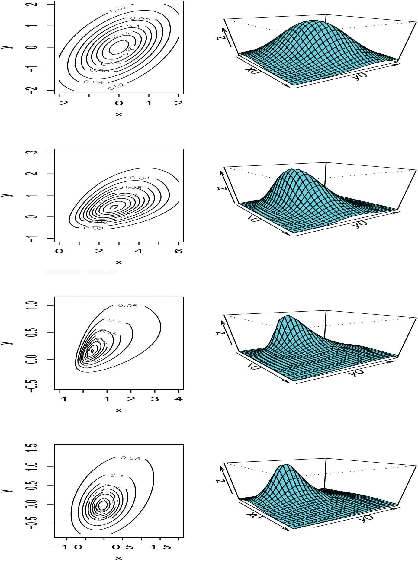
In the special case when
The mean vector and covariance matrix of
Table 1 represents the upper bounds of the measures of the skewness and kurtosis coefficients for the univariate SNMVBS under
| Measure | ||||||||||
|---|---|---|---|---|---|---|---|---|---|---|
| Skewness | 1.4547 | 2.6579 | 3.8459 | 4.4786 | 4.6996 | 4.7301 | 4.7619 | 4.7738 | 4.7826 | 4.7859 |
| Kurtosis | 6.8981 | 10.789 | 20.910 | 27.107 | 29.409 | 29.736 | 30.082 | 30.213 | 30.312 | 30.349 |
Upper bounds of the measures of skewness and kurtosis coefficients for the univariate SNMVBS under
Denoting by
The conditional distribution of
Using representation (8), after some algebra, we note that
Thus, we have
In Appendix A, we have established some theoretical properties and characteristics of SNMVBS distribution, including moment generating function, affine transformation, and conditional distributions. In the following theorem, conditional moments of
Theorem 2.2.
Let
The conditional PDF of
where- for
- for
Proof.
The conditional PDF in (11) can be obtained by using Bayes’ rule and some algebraic operations. The conditional expectation in (12) is obtained from Part (i) of the theorem and Part (ii) of Lemma Appendix A.1 in Appendix A. The conditional expectation in (13) is calculated directly.
To determine the parameter estimates of the SNMVBS distribution, we propose the Expectation-Maximization (EM)-type algorithms in the next section. The conditional expectations given in Theorem 2.2 become very useful for this purpose.
3. PARAMETER ESTIMATION
3.1. ECM Algorithm
Dempster et al. [18] introduced the EM algorithm technique as a versatile tool for ML estimation of models when there are missing data or latent variables. Simplicity in the implementation of the algorithm and the monotonic convergence are two most important features of the EM procedure. However, it is not directly applicable for estimating the parameters of the SNMVBS model because the M-step involves intractable computations. To avoid this problem, we use the Expectation-Conditional-Maximization (ECM) algorithm, suggested by Meng and Rubin [19], which replaces the M-step of the EM by a sequence of simpler conditional maximization steps.
Let
Then, under the hierarchical representation in (14), with
Now, to perform the ECM algorithm, we start with the E-step, given the current parameter
The
In summary, the ECM algorithm proceeds with the following steps:
E-step: Given the current value
CM-steps: Maximize (17), with respect to
We then update
The above procedure is repeated until either the maximum number of iterations is reached or a suitable stopping criterion is satisfied. Moreover, Appendix B details an approach for estimating the standard errors of the ML estimates using the observed information matrix.
3.2. Computational Strategies for the Implementation
One of the attractive properties of the EM-type algorithms is that successive iterates monotonically increase the likelihood value. So, a highly useful way to confirm convergence is that the difference between two successive log-likelihood values is less than a user-specified error tolerance. In this paper, we have used the Aitken acceleration method [20] to avoid the lack of process when determining the actual convergence [21]. Given the sequence of observed log-likelihood
Moreover, the implementation of EM algorithms requires initial values. Essentially, good initial values for the optimization process may speed up or even enable the convergence [22]. In our computations, we used the following method for choosing initial values. For
4. SIMULATION STUDY
To examine the performance of the proposed distribution as well as the estimation method, a small simulation study is carried out here. Through this emperical study, we examine the finite-sample properties of ML estimators obtained by the ECM algorithm, described earlier in Section 3. For this purpose, Monte Carlo samples of size
To examine the accuracies of parameter estimates, we computed the bias and the mean squared error (MSE), defined as
Furthermore, we computed the standard deviations of the ML estimates across 300 Monte Carlo samples (MC.SEs) and compared them with the average values of the approximate standard errors (A.SEs) obtained through the inverse of the observed information matrix, presented in Appendix B. Numerical results displayed in Tables 2 and 3 show the empirical consistency of the ML estimates as the Bias and MSE values both shrink toward zero when
| n = 50 |
n = 100 |
|||||||
|---|---|---|---|---|---|---|---|---|
| Parameter | Bias | MSE | MC.SE | A.SE | Bias | MSE | MC.SE | A.SE |
| −0.0531 | 0.2074 | 0.2599 | 0.2959 | −0.0189 | 0.1211 | 0.1704 | 0.1882 | |
| −0.0532 | 0.1905 | 0.2896 | 0.2918 | −0.0262 | 0.1237 | 0.1864 | 0.1890 | |
| −0.0603 | 0.3948 | 0.2709 | 0.2945 | −0.0321 | 0.2962 | 0.1943 | 0.1835 | |
| 0.1352 | 0.3642 | 0.1975 | 0.2705 | −0.0863 | 0.2424 | 0.1379 | 0.1697 | |
| −0.0728 | 0.4889 | 0.2821 | 0.2943 | −0.0616 | 0.3016 | 0.2029 | 0.1840 | |
| −0.0625 | 0.2375 | 0.3359 | 0.4935 | −0.0404 | 0.1784 | 0.2244 | 0.2886 | |
| −0.0715 | 0.2524 | 0.3028 | 0.4782 | −0.0574 | 0.1801 | 0.2442 | 0.2874 | |
| 0.0059 | 0.7948 | 0.7967 | 2.1740 | −0.0279 | 0.5528 | 0.5978 | 1.2770 | |
| 0.1124 | 0.8508 | 0.8944 | 2.1805 | 0.0856 | 0.5820 | 0.6199 | 1.2425 | |
| 0.0331 | 0.3653 | 0.4025 | 0.4939 | 0.0431 | 0.2364 | 0.2341 | 0.3085 | |
Simulation results for assessing the asymptotic properties of parameter estimates and standard errors, when n = 50 and 100.
| n = 200 |
n = 500 |
|||||||
|---|---|---|---|---|---|---|---|---|
| Parameter | Bias | MSE | MC.SE | A.SE | Bias | MSE | MC.SE | A.SE |
| −0.0086 | 0.0820 | 0.1135 | 0.1159 | −0.0041 | 0.0498 | 0.0762 | 0.0807 | |
| −0.0114 | 0.0882 | 0.1178 | 0.1183 | −0.0059 | 0.0530 | 0.0706 | 0.0807 | |
| −0.0121 | 0.2122 | 0.1293 | 0.1093 | −0.0147 | 0.1352 | 0.0903 | 0.0789 | |
| −0.0361 | 0.1682 | 0.0786 | 0.0958 | −0.0255 | 0.1009 | 0.0544 | 0.0617 | |
| −0.0160 | 0.2220 | 0.1407 | 0.1096 | −0.0146 | 0.1424 | 0.0973 | 0.0786 | |
| −0.0137 | 0.1298 | 0.1396 | 0.1633 | −0.0074 | 0.0745 | 0.0955 | 0.1098 | |
| −0.0247 | 0.1229 | 0.1493 | 0.1635 | −0.0156 | 0.0737 | 0.1018 | 0.1093 | |
| −0.0244 | 0.3842 | 0.3746 | 0.7025 | −0.0063 | 0.2333 | 0.2594 | 0.4891 | |
| 0.0361 | 0.4014 | 0.3862 | 0.6913 | 0.0252 | 0.2653 | 0.2497 | 0.4874 | |
| 0.0175 | 0.1667 | 0.1469 | 0.1792 | 0.0042 | 0.1016 | 0.1059 | 0.1229 | |
Simulation results for assessing the asymptotic properties of parameter estimates and standard errors, when n = 200 and 500.
5. APPLICATIONS
In this section, two applications of the SNMVBS distribution are presented. These examples come from environmental studies in a multivariate setting and possessing some outliers. In these cases, the SNMVBS distribution provides a better fit to these data than the other skewed models mentioned earlier.
5.1. Wind Speed Data
In this example, we consider the wind speed dataset and then fit the SNMVBS distribution in its multivariate form. The wind speed dataset consists of
Here, we fit the SNMVBS distribution for these data as an alternative model. Figure 2 shows classical and robust Mahalanobis distances of this bivariate data. The plots show some outliers in these data and consequently a symmetric distribution will not be a good choice in this case. We assume (gh, kw) as a two-dimensional vector and fit a bivariate SNMVBS to that. Similarly, we also fit bivariate NIG, ST, and NMVBS distributions for the sake of comparison. As recommended by an anonymous referee, we also fitted the skew-Laplace distribution, known as shifted asymmetric Laplace (SAL), introduced by Franczak et al. [24]. The SAL random variable can be represented by (1) when
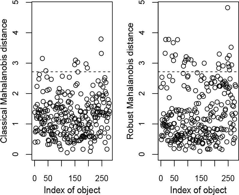
Wind speed data: Classical and robust Mahalanobis distances.
| Par | SNMVBS | ST | NMVBS | NIG | SAL |
|---|---|---|---|---|---|
| 25.41 (2.639) | 28.48 (0.652) | 32.68 (10.49) | 33.80 (4.526) | 23.07 (1.145) | |
| 40.94 (7.584) | 24.09 (1.018) | 40.09 (14.06) | 41.10 (5.527) | 22.01 (2.730) | |
| 424.25 (41.25) | 387.45 (5.397) | 97.97 (31.09) | 94.10 (24.03) | 136.26 (18.47) | |
| 213.68 (40.57) | 241.45 (3.590) | 30.36 (39.15) | 20.07 (25.26) | 85.24 (19.01) | |
| 259.45 (43.36) | 349.09 (2.822) | 183.84 (52.54) | 188.35 (38.59) | 345.65 (35.35) | |
| 3.24 (2.521) | - | −18.33 (10.42) | −21.06 (4.573) | −10.32 (1.285) | |
| −18.37 (7.180) | - | −23.95 (14.15) | −27.07 (5.731) | −7.97 (2.759) | |
| −5.54 (0.448) | −4.48 (0.180) | - | - | - | |
| −1.16 (0.347) | −0.10 (0.299) | - | - | - | |
| 0.38 (0.073) | 17.62 (0.121) | 0.41 (0.154) | 5.08 (0.006) | - | |
| −2228.43 | −2237.54 | −2244.43 | −2244.35 | −2257.33 | |
| AIC | 4476.86 | 4491.08 | 4504.86 | 4504.71 | 4528.66 |
| BIC | 4513.14 | 4520.11 | 4533.88 | 4533.73 | 4554.05 |
| HQIC | 4491.37 | 4502.73 | 4516.55 | 4516.36 | 4538.85 |
Estimation results and information criteria for wind speed data (gh, kw). Standard errors of ML estimates are given in parentheses.
Performance assessments for studied models were made on the adequacy of overall fitness in terms of the Akaike Information Criterion (AIC; [25]), Bayesian Information Criterion (BIC; [26]) and Hannan–Quinn information Criterion (HQIC; [27]), defined as
As can be seen from Table 4, it is evident from the AIC, BIC, and HQIC values that the SNMVBS model provides the best fit for these data. Figure 3 presents the scatter plots of wind data along with the contour plots of the fitted density and the fitted density function of the SNMVBS distribution. The plots reveal that the SNMVBS distribution can effectively capture the skewness and heavy-tails present in the data.
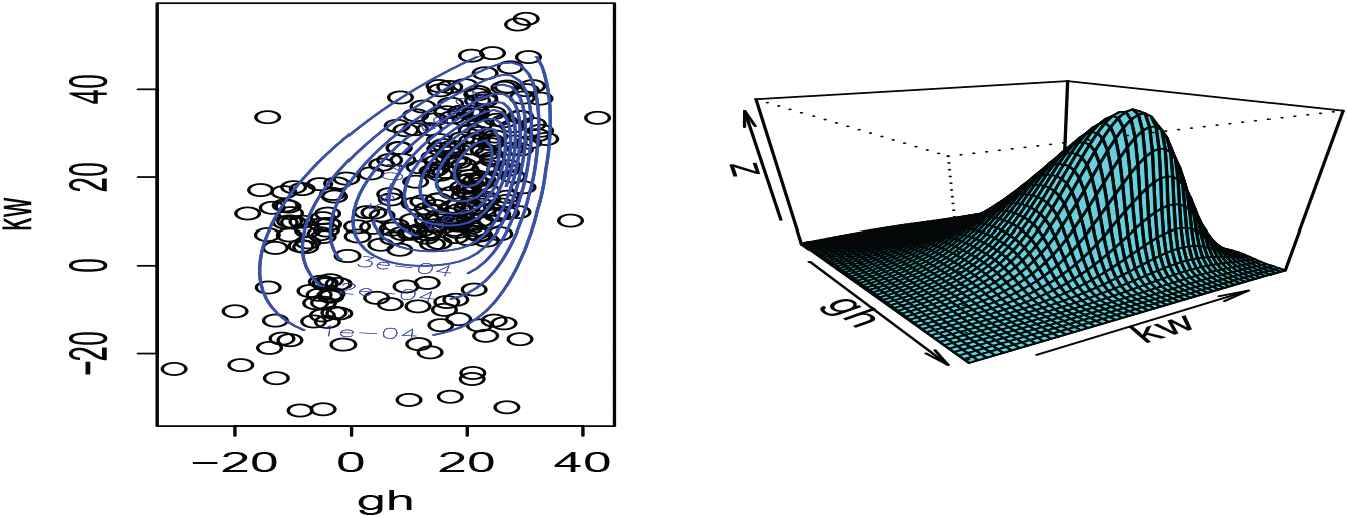
Wind speed data: Scatter plot (gh, kw) with fitted density contours and the fitted density of the skew-normal mean-variance mixture based on Birnbaum–Saunders (SNMVBS) distribution.
5.2. Water Quality Data
Cook and Johnson [28] introduced a new distribution and investigated its application in water quality. These data consist of log concentrations of seven chemical elements in 655 water samples collected near Grand Junction in Western Colorado. Concentrations were measured for the following elements: Uranium (U), Lithium (Li), Cobalt (Co), Potassium (K), Cesium (Cs), Scandium (Sc), and Titanium (Ti). The data are presented in package “copula.” Figure 4 shows that there are some potential outliers in these data. The estimates of parameters are not shown here, but Figures. 5 and 6 show the contour plots of pairs of variables with multivariate SNMVBS contours. Clearly, the SNMVBS distribution provides a good fit for these data. Table 5 presents the information criteria of some alternate models. From this table, we observe once again that the AIC, BIC, and HQIC of SNMVBS are the lowest among all considered models.
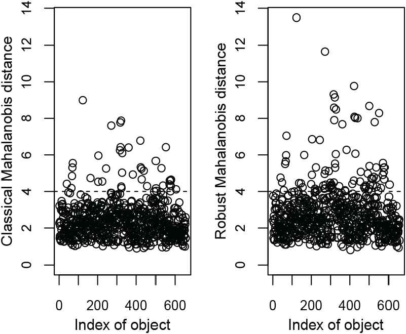
Water quality data: Classical and robust Mahalanobis distances.
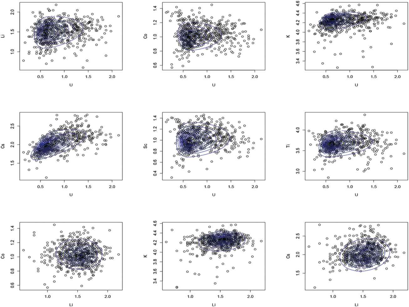
Water quality data: Scatter plots with superimposed fitted skew-normal mean-variance mixture based on Birnbaum–Saunders (SNMVBS) density contours for some concentrations.
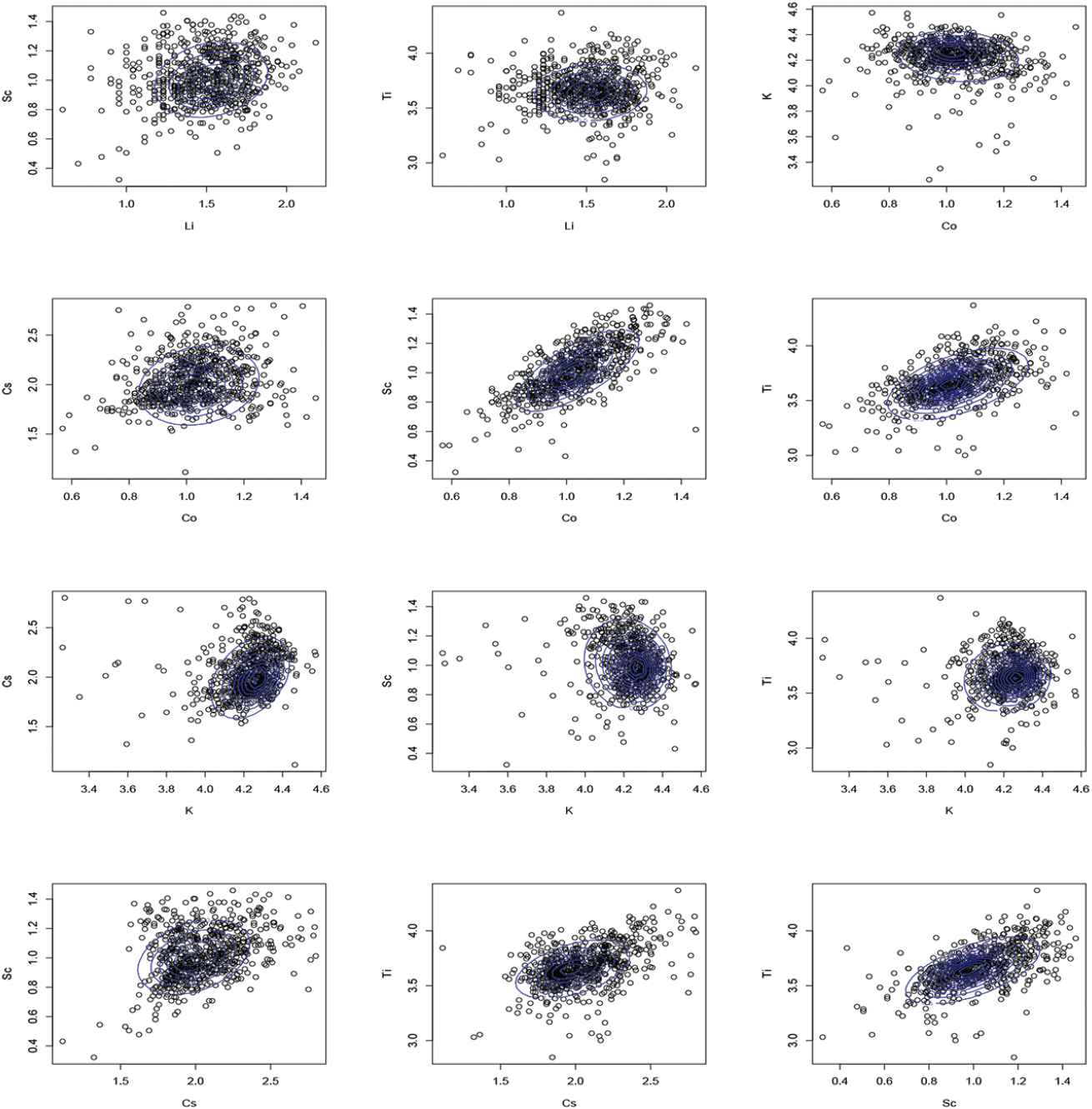
Water quality data: (Continued).
| Criterion | SNMVBS | ST | NMVBS | NIG | SAL |
|---|---|---|---|---|---|
| 1969.61 | 1923.66 | 1925.58 | 1926.93 | 1839.19 | |
| AIC | −3839.20 | −3761.33 | −3765.16 | −3767.86 | −3594.39 |
| BIC | −3614.96 | −3568.49 | −3572.32 | −3575.02 | −3406.04 |
| HQIC | −3752.26 | −3686.57 | −3690.75 | −3693.09 | −3521.36 |
Water quality data: maximum log-likelihood, AIC, and BIC for different fitted models.
6. CONCLUDING REMARKS
We have introduced in this work a multivariate skew-normal mean-variance mixture distribution obtained by employing BS as a mixing distribution. The properties of the SNMVBS distribution are studied, and a feasible EM-type algorithm for estimating parameters has been developed. We have demonstrated our methodology with a simulation study and have shown that the SNMVBS model outperforms other skew models in two data sets. The proposed distribution has some desirable properties. It offers a flexible class of distributions for modeling skewed and heavy-tailed data. It also provides a good fit to data consisting of outliers. Moreover, in contrast to the ST model, estimates of all parameters of the SNMVBS distribution can be obtained by solving some simple linear equations in the proposed ECM algorithm.
ACKNOWLEDGMENTS
We gratefully acknowledge the associate editor and three anonymous referees for their valuable comments and suggestions, which led to this greatly improved version of the article. We are also grateful to Prof. Tsung-I Lin for his help on the earlier version of the paper.
APPENDIX A. THEORETICAL PROPERTIES
The following lemmas are useful in establishing some properties of the skew-normal mean-variance mixture based on Birnbaum–Saunders (SNMVBS) distribution.
Lemma A.1.
If
Parts (i) and (ii) of the above lemma are well-known properties of generalized inverse Gaussian (GIG) distribution; see [7] for details. Part (iii) has been proved by [12].
Lemma A.2.
Let
The probability density function (PDF) of
In particular, we have
The proof of Lemma A.2 and some other useful properties of BS can be found in Leiva [15], for example.
We now present the proof of Theorem 2.1.
Proof.
From (6), we have
The following proposition presents the moment generating function (mgf) of Y.
Proposition A.1.
The mgf of
Proof.
The proof is completed by performing some algebraic calculations.
The next theorem shows that SNMVBS random vector is invariant under linear transformations. Also, the marginal distributions of SNMVBS are presented.
Theorem Appendix A.1.
Let
Foy any
Suppose Y is partitioned as
Then,
Proof.
The proof of Part (i) is straightforward by obtaining the mgf of
Although there is no closed-form for the conditional distribution of SNMVBS distribution, it is clear that the conditional distribution of
APPENDIX B. PROVISION OF STANDARD ERRORS
To compute the asymptotic covariance of the maximum likelihood (ML) estimates, we use the method suggested by Basford et al. [29]. Let
The standard errors of ML estimates can then be found by calculating the square root of the diagonal elements of
The
REFERENCES
Cite this article
TY  - JOUR
AU  - M. Tamandi
AU  - N. Balakrishnan
AU  - A. Jamalizadeh
AU  - M. Amiri
PY  - 2019
DA  - 2019/07/03
TI  - A Multivariate Skew-Normal Mean-Variance Mixture Distribution and Its Application to Environmental Data with Outlying Observations
JO  - Journal of Statistical Theory and Applications
SP  - 244
EP  - 258
VL  - 18
IS  - 3
SN  - 2214-1766
UR  - https://doi.org/10.2991/jsta.d.190617.001
DO  - 10.2991/jsta.d.190617.001
ID  - Tamandi2019
ER  -