Journal of Statistical Theory and Applications

Volume 17, Issue 4, December 2018, Pages 674 - 685

On Properties and Applications of a Two-Parameter Xgamma Distribution

Authors
Subhradev Sen1, *, N. Chandra2, Sudhansu S. Maiti3
1Alliance School of Business, Alliance University, Bengaluru, Karnataka, India
2Department of Statistics, Pondicherry University, Kalapet, Puducherry, India
3Department of Statistics, Visva-Bharati University, West Bengal, India
*

Corresponding author. Email: subhradev.stat@gmail.com

Received 10 January 2017, Accepted 11 February 2018, Available Online 31 December 2018.
DOI
10.2991/jsta.2018.17.4.9How to use a DOI?
Keywords
Lifetime distribution; maximum likelihood estimation; survival properties; reliability;
Abstract

An existing one-parameter probability distribution can be very well generalized by adding an extra parameter in it and, in turn, the two-parameter family of distributions, thus obtained, provides added flexibility in modeling real life data. In this article, we propose and study a two-parameter generalization of xgamma distribution [1] and utilize it in modeling time-to-event data sets. Along with the different structural and distributional properties of the proposed two-parameter xgamma distribution, we concentrate in studying useful survival and reliability properties, such as hazard rate, reversed hazard rate, stress-strength reliability etc. Two methods of estimation, viz. maximum likelihood and method of moments, are been suggested for estimating unknown parameters. Distributions of order statistics, stochastic order relationships are investigated for the proposed model. A Monte-Carlo simulation study is carried out to observe the trends in estimation process. Two real life time-to-event data sets are analyzed and the proposed model is compared with some other two-parameter lifetime models in the literature.

Copyright
© 2018 The Authors. Published by Atlantis Press SARL.
Open Access
This is an open access article under the CC BY-NC license (http://creativecommons.org/licences/by-nc/4.0/).

1. INTRODUCTION

Adding extra parameters to an existing family of distributions is very common in the statistical distribution theory as the resulting family of distributions, thus obtained, becomes richer and sometimes more flexible in modeling real life data sets. However, adding more parameters to an existing family of distributions may create complications in its basic structural properties and/or in methods of estimating the additional parameters, see for more details Johnson et al. [2]. Nevertheless, adding an extra parameter to an existing probability distribution generalizes the baseline distribution and provides flexibility in modeling or describing real life data.

Recently, Sen et al. [1] introduced and studied a one-parameter lifetime distribution, named as xgamma distribution, with probability density function (PDF) as

fx=θ21+θ1+θ2x2eθx,x>0,θ>0.
The xgamma distribution has several interesting structural and survival properties that made it useful in modeling time-to-event data sets. In another recent research paper, Sen and Chandra [3] introduced and studied different properties of a two-parameter extension or generalization of xgamma density, named as quasi xgamma distribution (QXD), and applied it in modeling bladder cancer survival data. QXD resembles closely with xgamma distribution in its density form and in other survival properties.

Our objective in this article is to introduce and study an another two-parameter generalization of xgamma distribution by adding an additional parameter α(>0) to it. The beauty of this two-parameter extension is that it contains xgamma distribution as a special case. We have studied different distributional, survival and/or reliability properties of this two-parameter xgamma distribution (TPXG) and demonstrated its applicability in modeling lifetime data sets with potential flexibility over existing two-parameter lifetime models. The rest of the article is organized as follows:

The TPXG along with its alternative form is introduced in section 2. The moments and related measures are studied in section 3. Incomplete moments are utilized in studying famous inequality curves and different entropy measures are studied in sections 4 and 5, respectively. In section 6, different survival properties are studied. Stress-strength reliability and distributions of order statistics are described in sections 7 and 8, respectively. Section 9 studies some stochastic ordering. Methods of estimating parameters are discussed in section 10. A sample generation algorithm along with a Monte-Carlo simulation study is presented in section 11. In section 12, two real data sets are analyzed to show the applicability of TPXG. Finally, section 13 concludes.

2. THE TPXG

In this section we introduce and study a two-parameter form of the xgamma distribution. We have the following definition.

Definition 2.1.

A continuous random variable, X, will be said to follow a TPXG with parameters α and θ if its PDF is of the form

fx=θ2α+θ1+αθ2x2eθx,x>0,θ>0,α>0.
We denote it by XTPXGα,θ.

Note.

  1. When we put α=1 in (2), we obtain the xgamma distribution with parameter θ as a special case.

  2. The TPXG as obtained in (2) is a special mixture of exponential(θ) and gamma (3,θ) with mixing proportions θ/α+θ and α/α+θ, respectively.

Alternative form:

An alternative form of the TPXG can be obtained by putting β=1/α in (2) and will have the form of the PDF as

fx=θ21+βθβ+θ2x2eθx,x>0,θ>0,β>0.
The cumulative distribution function (CDF) of X as given in 2 is given by
Fx=1α+θ+αθx+12αθ2x2α+θeθx,x>0,θ>0,α>0.
The characteristic function (CF) of X is derived as
ϕXt=EeitX=θ2α+θ(θit)1+αθ(θit)3;t,i=1.
The plot of probability density curves for different values of α and θ is shown in Fig. 1.

Figure 1

Probability density function of two-parameter xgamma distribution for different values of α and θ.

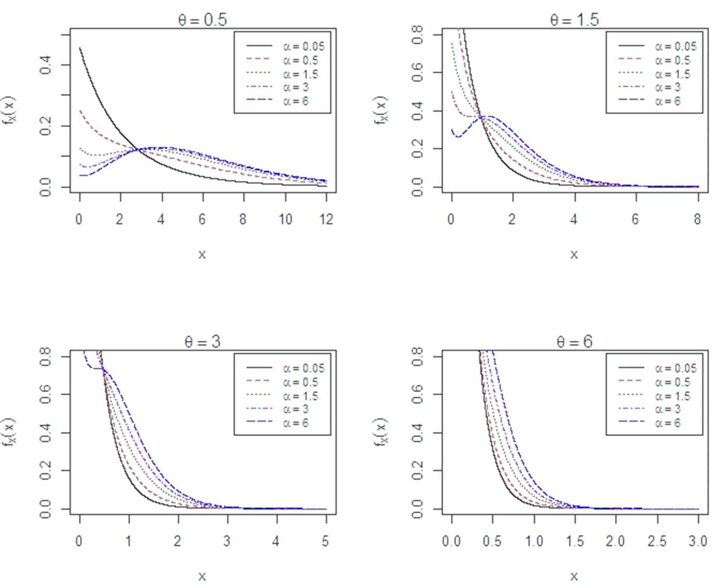
3. MOMENTS AND RELATED MEASURES

In this section we study the moments and other related measures for the TPXG with parameters α and θ, i.e., TPXGα,θ.

The rth order raw moments for XTPXGα,θ is obtained as

μr=EXr=0xrθ2α+θ1+αθ2x2eθxdx=r!2θrα+θ2θ+α1+r2+r;r=1,2,.
In particular, we have,
μ1=EX=θ+3αθα+θ;μ2=EX2=2θ+6αθ2α+θ.
So, we have the expression for second order central (about mean) moment or the population variance for X as
VX=μ2=2θ2+8αθ+3α2θ2(α+θ)2
so that the coefficient of variation (CV) becomes
γ=2θ2+8αθ+3α2θ+3α.

The moment generating function (MGF) of X is derived as

MXt=EetX=θ2α+θ(θt)1+αθ(θt)3;t.
The cumulant generating function (CGF) of X is obtained as
KXt=lnMXt=lnθ2α+θθt+ln1+αθ(θt)2;t.
The following theorem shows that TPXGα,θ is unimodal.

Theorem 3.1.

For θ>α/2, the PDF, fx of XTPXGα,θ, as given in (2), is decreasing in x.

Proof. We have from (2) the first derivative of fx with respect to x as

fx=θ2α+θαθxθ12αθ2x2eθx.
f(x) is negative in x when θ>α/2, and hence the proof.

So, we have from the theorem 3.1, for θα/2, ddxfx=0 which implies that 1+12θα/θ is the unique critical point at which fx is maximized.

Hence, the mode of TPXGα,θ is given by

ModeX=1+12θαθ,if 0<θα/2.0,otherwise.

4. INCOMPLETE MOMENTS AND INEQUALITY CURVES

The rth incomplete moment, μrt (say), for a random variable X with PDF fx is defined as

μrt=0txrfxdx
When XTPXGα,θ, the rth incomplete moment is obtained as
μrt=θ2α+θ0txr1+αθ2x2eθxdx=θ2α+θγr+1,θt+αθ2γr+3,θt,
where γa,x=0xua1eudu is lower incomplete gamma function.

Lorenz curve and Bonferroni curve are well known inequality curves (see for more details Kleiber and Kotz [4]) that have been extensively applied in many fields such as economics, demography, insurance, medicine and reliability engineering.

When a non-negative continuous random variable X has PDF fx and CDF Fx, the Lorenz and Bonferroni curves are defined by

Lp=1μ0qxfxdx
and
Bp=1pμ0qxfxdx
respectively, where μ=EX and q=F1p for 0<p<1.

When XTPXGα,θ, we use the first incomplete moment putting r=1 in (14) to obtain Lorenz and Bonferroni curves as

Lp=θ33α+θγ2,θq+αθ2γ4,θq
and
Bp=θ3p3α+θγ2,θq+αθ2γ4,θq,
respectively, where, for given p, α and θ, q is the solution of the equation, γ1,θq+αθ2γ3,θq=pα+θθ2 that can easily be solved numerically.

5. ENTROPY MEASURES

An entropy of a random variable X is a measure of variation of the uncertainty. A popular entropy measure is Rényi entropy. If a non-negative continuous random variable, X, has the PDF fx, then Rényi entropy is defined as

HRγ=11γln 0fγxdxforγ>01.

When XTPXGα,θ, one can derive

0fγxdx=θ2γ(α+θ)γj=0γγjα2jΓ2j+1θj+1γ2j+1
to obtain Rényi entropy as
HRγ=11γ2γln θγln (α+θ)+11γln j=0γγjα2jΓ2j+1θj+1γ2j+1.
In physics, the Tsallis entropy[5] is a generalization of the standard Boltzmann-Gibbs entropy. For an absolutely continuous non-negative random variable X with PDF fx, Tsallis entropy (also called q-entropy) is definedas
SqX=1q1ln10fqxdxfor q>01
When XTPXGα,θ, Tsallis entropy can be derived as
Sq(X)=1q1ln[1θ2q(α+θ)qj=0q(qj)(α2)jΓ(2j+1)θj+1q2j+1].
Shannon measure of entropy is defined as
Hf=Eln fx=0ln fxfxdx.
For XTPXGα,θ, Shannon entropy is obtained as
H(f)=(3α+θα+θ)lnθ2(α+θ)θ2(α+θ)j=1(1)j+1(α/2)jθj+1j[Γ(2j+1)+α2θΓ(2j+3)].

6. SURVIVAL PROPERTIES

In this section we study different survival properties of the TPXG with parameters α and θ given in (2).

The survival function (SF) of X is given by

Sx=α+θ+αθx+12αθ2x2α+θeθx;x>0,θ>0,α>0.
The hazard rate (HR) function of X is obtained as
hx=fxSx=θ21+αθ2x2α+θ+αθx+12αθ2x2;x>0,θ>0,α>0.

Note. The HR function, hx, is increasing for x>2αθ (see Fig. 2 for HR plot for different values of α and θ) with the following bounds.

Figure 2

Hazard rate function of two-parameter xgamma distribution for different values of α and θ.

f0=θ2α+θ<hx<θ

Theorem 6.1.

The failure rate, hx, as given in (21) is increasing failure rate (IFR) in distribution for x>2αθ and is decreasing failure rate (DFR) in distribution for x<2αθ.

Proof. The proof comes immediately as the PDF given in (2) is log-concave for x>2αθ and log-convex for x<2αθ.

The reversed hazard rate (RHR) function of X is obtained as

rx=fxFx=θ21+αθ2x2eθxα+θ1eθx1+θx2αθxeθx;x>0,θ>0,α>0.
The mean residual life (MRL) function of X is given by
mx=EXx|Xx=1SxxStdt=1θ+α2+θxθα+θ+αθx+12αθ2x2.

Note. The MRL function, mx, is bounded with the following limits,

1θ<mx<θ+3αθα+θ=EX.

7. STRESS-STRENGTH RELIABILITY

Let X and Y be continuous random variables denote strength and stress, respectively, of an equipment or a system, then the stress-strength reliability is defined as

R=PrX>Y=0PrX>Y|Y=yfYydy=0SXyfYydy,
where fY. is the PDF of Y and SX. is the SF of X.

If XTPXGα1,θ1 and YTPXGα2,θ2 independently, then stress-strength reliability is obtained as

R=θ22(α1+θ1)(α2+θ2)[(α1+θ1θ1+θ2)+α1θ1(θ1+θ2)2+α1α2θ2+α2θ1θ2+α1θ12(θ1+θ2)3]+3α1α2θ1θ23(α1+θ1) (α2+θ2(θ1+θ2)4+6α1α2θ12θ23(α1+θ1) (α2+θ2(θ1+θ2)5.
In particular, when X and Y are independently and identically distributed (IID) TPXGα,θ, we have the expression for stress-strength reliability as
R=θ2(α+θ)2αθ+12+α22θ2

Note. If we put α=1 in (25), we have R=1/2, which is nothing but the stress-strength reliability when X and Y are IID xgammaθ.

8. DISTRIBUTION OF ORDER STATISTICS

Distributions of order statistics for a lifetime random variable play important roles in computing system reliability in case of series or parallel configurations with IID components.

Let X1,X2,,Xn be a random sample of size n drawn from XTPXGα,θ.

Denote Xj as the jth order statistic. Then X1 and Xn denote the smallest and largest order statistics for a sample of size n drawn from TPXGα,θ, respectively.

The PDF of X1 is derived as

fX1x=n1Fxn1fx=nθ2(α+θ)n1+αθ2x2α+θ+αθx+12αθ2x2n1enθx
for x>0, θ>0 and α>0.

Similarly, the PDF of Xn is obtained as

fXnx=n[Fx]n1fx=nθ2(α+θ)n1+αθ2x2α+θ1eθx1+θx2αθxeθxn1eθx
for x>0, θ>0 and α>0.

9. STOCHASTIC ORDERING

In this section we study stochastic ordering relations for random variables following TPXGα,θ. Stochastic ordering is an important tool for judging the comparative behavior. Recall some basic definitions.

Definition 9.1.

A non-negative random variable X1 is said to be smaller than an another non-negative random variable X2 in the

  1. stochastic order X1STX2 if FX1xFX2x for all x.

  2. HR order X1HRX2 if hX1xhX2x for all x.

  3. MRL order X1MRLX2 if mX1xmX2x for all x.

  4. likelihood ratio order X1LRX2 if fX1xfX2x decreases in x.

The following implications [6] are well justified:

X1LRX2X1HRX2XMRLX2 and
XHRX2XSTX2.
The following theorems shows that the TPXG is ordered with respect to the strongest likelihood ratio ordering and thereby the other orderings as mentioned in definition 9.1.

Theorem 9.1.

Let X1TPXGα1,θ1 and X2TPXGα2,θ2. If α1=α2 and θ1θ2 (or, if θ1=θ2 and α1α2), then X1LRX2 and hence X1HRX2, X1MRLX2 and X1STX2.

Proof. Let us denote the PDF of X1 as fX1x and that of X2 be fX2x for x>0.

We have then the ratio

fX1xfX2x=θ12α2+θ2θ22α1+θ11+α1θ12x21+α2θ22x2eθ1θ2x
Taking logarithm both sides, we have
lnfX1xfX2x=2lnθ1θ2+lnα2+θ2α1+θ1+ln1+α1θ12x21+α2θ22x2θ1θ2x.

The first derivative with respect to x gives

ddxlnfX1xfX2x=α1θ1α2θ2x1+α1θ12x21+α2θ22x2θ1θ2,
which is negative when α1=α2 and θ1θ2 (or, when θ1=θ2 and α1α2), i.e., fX1xfX2x decreases in x when α1=α2 and θ1θ2 (or, when θ1=θ2 and α1α2), so X1LRX2 and the other orderings follow automatically by (28). Hence the proof.

Now, we establish stochastic order relationships between two random variables, X and Y, when XTPXGα1,θ1 and YQXDα2,θ2. Note that the QXD with parameters α and θ has the PDF

fx=θ1+αα+θ22x2eθx;x>0,α,θ>0
We have the following theorem.

Theorem 9.2.

Let XTPXGα1,θ1 and YQXDα2,θ2. If α1=α2=α(say), then XLRY whenever θ1θ2+θ22θ1α2 and θ1>θ2. Again, if θ1=θ2=θ(say), then XLRY whenever α1θα2.

Proof. The proof comes immediately following the similar arguments as followed in the proof of theorem 29. Hence is omitted.

10. ESTIMATION OF PARAMETERS

In this section we propose method of moments and maximum likelihood estimators (MLEs) for and θ when XTPXGα,θ.

Let X1,X2,,Xn be a random sample of size n drawn from α,θ. Denote X¯ as sample mean.

10.1. Method of Moments Estimation

Using the first two raw moments given in (7), we have

μ22μ1=2(θ+6α)(α+θ)(θ+3α)2=k(say)
Taking θ=cα, we have
μ22μ1=2c+6c+1(c+3)2=k
which give a quadratic equation in c as
2kc2+146kc+129k=0
An estimate of k is easily obtained by replacing μ1 and μ2 by sample moments X¯ and m2, respectively, in equation (29). This estimate can then be utilized to solve (30) to obtain an estimate of c. Again, from the first moment equation, we have
X¯=c+3αcc+1
and thus moment estimator of α, α˜ (say), is given by
α˜=c+3cc+11X¯.
Finally, the moment estimator, θ˜ (say), of θ is obtained as
θ˜=c+3c+11X¯.

10.2. Maximum Likelihood Estimation

Let x=x1,x2,,xn be n observations or realizations on a random sample X1,X2,,Xn of size n drawn from XTPXGα,θ. We have the likelihood function as

L(α,θ|X)=i=1nθ2(α+θ)(1+αθ2xi2)eθxi=θ2n(α+θ)neθi=1nxii=1n(1+αθ2xi2).
The log-likelihood function is given by
lnL(α,θ|x)=2nlnθnln(α+θ)θi=1nxi+i=1n1+αθ2xi2.
To find out the MLEs, α^ and θ^, of α and θ, we have two log-likelihood equations as
ln Lα,θ|xα=i=1nθ2xi21+αθ2xi2nα+θ=0
and
lnL(α,θ|x)θ=2nθn(α+θ)+i=1n(α2xi21+αθ2xi2)i=1nxi=0,
respectively.

Though the log-likelihood equations cannot be solved analytically, we can utilize numerical method for solving (34) and (35) to obtain the MLEs, α^ and θ^, respectively.

11. SAMPLE GENERATION AND SIMULATION STUDY

This section deals with the random sample generation algorithm for generating random samples of specific size from the TPXG. We make use of the fact that the distribution as given in (2), is a special mixtures of exponential (θ) and gamma (3,θ) for describing sample generation algorithm. To generate a random sample of size n from TPXGα,0a, we have the following simulation algorithm:

  1. Generate Uiuniform0,1,i=1,2, ,n.

  2. Generate Viexponentialθ,i=1,2, ,n.

  3. Generate Wigamma3,θ,i=1,2, ,n.

  4. If Uiθα+θ, then set Xi=Vi, otherwise, set Xi=Wi.

A Monte-Carlo simulation study was carried out considering N = 10000 times for selected values of n, α and θ. Samples of sizes 20, 30, 50, 80 and 100 were considered and values of α,θ were taken as 0.5,0.5, 1.5,2.0 and 3.0,4.0.

The following measures were computed:

  1. Average mean square error (MSE) of the simulated estimates α^i, i=1,2,,N:

    α^=1Ni=1N(α^iα)2

  2. Average MSE of the simulated estimates θ^i, i=1,2,,N:

    θ^=1Ni=1N(θ^iθ)2

The results of the simulation study are shown in Table 1. The following observations are made from the simulation study:

  1. The estimates of α and θ get closer to the corresponding true values as the sample size, n, increases.

  2. The average MSEs for estimates of α and estimates θ decrease with increasing sample size.

12. APPLICATION WITH REAL LIFE DATA ILLUSTRATION

In this section we analyze two different time-to-event data sets for illustrating the applicability of TPXG. For comparison purpose, besides TPXG, we consider five other two parameter lifetime distributions, viz., gamma distribution with shape α and rate θ, weibull distribution with shape α and scale β, log-normal distribution with parameters μ and σ, two-parameter Lindley distribution (TPLD) with parameters alpha and λ(Shanker et al. [7] and QXD with parameters α and θ [3].

α=0.1,θ=0.5
n α^ MSE of α^ θ^ MSE of θ^
20 0.3621 1.3402 0.6597 0.8742
50 0.2106 1.2201 0.5892 0.6420
80 0.1976 1.1046 0.5108 0.5602
100 0.1691 1.0042 0.5032 0.4763
α=0.1,θ=1.5
n α^ MSE of α^ θ^ MSE of θ^
20 0.3986 1.8756 1.6942 0.8966
50 0.2654 1.4320 1.5730 0.7021
80 0.1976 1.2205 1.5107 0.4503
100 0.1430 0.9986 1.5002 0.3064
α=1.5,θ=0.5
n α^ MSE of α^ θ^ MSE of θ^
20 2.0166 2.3106 0.6879 0.9845
50 1.9822 1.9658 0.5983 0.6650
80 1.7043 1.4576 0.5127 0.4501
100 1.6503 1.1212 0.5026 0.3326
α=1.5,θ=2.5
n α^ MSE of α^ θ^ MSE of θ^
20 2.1551 3.2249 2.6158 0.5344
50 1.9256 1.8867 2.5310 0.2776
80 1.8282 1.4404 2.5100 0.2047
100 1.7675 1.2444 2.5004 0.1753
α=3.0,θ=5.0
n α^ MSE of α^ θ^ MSE of θ^
20 4.6542 2.4328 5.7643 1.2376
50 4.1035 2.0122 5.3066 1.0544
80 3.6479 1.8768 5.1006 0.8790
100 3.4509 1.0256 5.0016 0.6504
Table 1

Estimates and average MSEs of α and θ for different sample sizes.

In order to compare the two distribution models, we consider criteria like, -log-likelihood, AIC (Akaike information criterion, see [8]) and BIC (Bayesian information criterion, see [9]), for the data sets. The better distribution corresponds to smaller -log-likelihood, AIC and BIC values. MLE is used for estimating the model parameters for both the data sets.

Illustration I: As a first illustration we consider a data set on the failure times of an electronic device reported in Wang [10]. Table 2 represents the data of 18 failure times of an electronic device. Table 3.

5 11 21 31 46 75 98 122 145 165 196 224 245 293 321
330 350 420
Table 2

Time to failure of 18 electronic devices.

shows the estimates of the model parameter(s) with standard error(s) of estimates in parenthesis and model selection criteria for the first data set.

Distributions Estimate(Std. Error) -Log-likelihood AIC BIC
Gammaα,θ α^=1.11310.3206
θ^=0.00640.0022 2110.60 2225.21 2226.99
Weibullα,β α^=1.14580.2287
β^=179.6938.6837 2110.45 2224.89 2226.67
Log-normalμ,σ μ^=4.63580.2952
σ^=1.25230.2087 2113.03 2230.07 2231.85
TPLDα,λ α^=0.00900.0134
λ^=0.00870.0024 2110.30 2224.59 2226.37
QXDα,θ α^=0.72510.5740
θ^=0.01250.0027 2110.24 2224.48 2226.26
TPXGα,θ α^=0.01730.0158
θ^=0.01250.0027 2109.62 2223.25 2225.03
Table 3

MLEs of model parameters and model selection criteria for failure times data of 18 electronic devices.

Illustration II: As a second illustration we consider a data set on the lifetimes of a device reported in Aarset [11]. Table 4. represents the data of 50 lifetimes of a device.

0.1 0.2 1 1 1 1 1 2 3 6 7 11 12 18 18
18 18 18 21 32 36 40 45 46 47 50 55 60 63 63
67 67 67 67 72 75 79 82 82 83 84 84 84 85 85
85 85 85 86 86
Table 4

Lifetimes of 50 devices.

Table 5 shows the estimates of the model parameter(s) with standard error(s) of estimates in parenthesis and model selection criteria for the data set represented in Table 4.

In each of the above illustration, TPXGα,θ provides better fit (in view of -log-likelihood, AIC and BIC values) as compared to the well-known lifetime models for the considered data set. Hence, the two-parameter extension of xgamma distribution provides flexibility in modeling real life data sets in comparison with other two-parameter lifetime distributions in the literature.

Distributions Estimate(Std. Error) -Log-likelihood AIC BIC
Gammaα,θ α^=0.79900.1375
θ^=0.01750.0041 2240.19 2484.38 2488.20
Weibullα,β α^=0.94920.1196
β^=44.91946.9458 2241.00 2486.00 2489.83
Log-normalμ,σ μ^=3.07900.2472
σ^=1.74810.1748 2252.82 2509.65 2513.47
TPLDα,λ α^=0.02560.0224
λ^=0.03170.0053 2240.16 2484.33 2488.15
QXDα,θ α^=0.70220.2984
θ^=0.04760.0056 2237.12 2478.24 2482.06
TPXGα,θ α^=0.06770.0330
θ^=0.04760.0056 2236.73 2477.47 2481.29
Table 5

MLEs of model parameters and model selection criteria for data on lifetimes of 50 devices.

13. CONCLUDING REMARKS

An extra non-negative parameter is added to an existing distribution, the xgamma distribution, for studying the different properties and applications of the extended distribution, named as TPXG. There are several other standard and well established procedures in the literature for obtaining generalized two-parameter family of distributions that include baseline distribution as a special case. This article reflects one such alternative in adding extra parameter to the xgamma distribution for the purpose of generalizing the baseline density and to study the general fact of added flexibility in modeling real life data sets without sacrificing much in standard estimation process. Although the article focuses in observing additional flexibility of the proposed two-parameter xgamma model over the standard two-parameter models in modeling time-to-event data sets, the proposed model might also be useful and potential in describing data sets coming from diverse areas of application owing to the fact of its lucrative structural and/or distributional properties and easy standard estimation aspects.

REFERENCES

1.S. Sen, S.S. Maiti, and N. Chandra, The xgamma distribution: Statistical properties and application, J. Mod. Appl. Stat. Methods., Vol. 15, No. 1, 2016, pp. 774-788.
2.N.L. Johnson, S. Kotz, and Balakrishnan, N. Continuous Univariate Distributions,, John Wiley & Sons, New York, Vol. 1, 1994.
3.S. Sen and N. Chandra, The quasi xgamma distribution with application in bladder cancer data, Journal of Data Science, Vol. 15, No. 1, 2017, pp. 61-76.
4.C. Kleiber and S. Kotz, S, Statistical Size Distributions in Economics and Actuarial Sciences,, John Wiley & Sons, New York, Vol. 470, 2003.
5.C. Tsallis, Possible generalization of Boltzmann-Gibbs statistics, J. Stat. phys., Vol. 52, No. 1-2, 1988, pp. 479-487.
6.M. Shaked and J.G. Shanthikumar, Stochastic Orders and Their Applications, Academic Press, 1994.
7.R. Shanker, S. Sharma, and R. Shanker, A two-parameter Lindley distribution for modeling waiting and survival times data, Appl. Math., Vol. 4, No. 02, 2013, pp. 363-368.
8.H. Akaike, A new look at the statistical model identification, IEEE trans. Automat. Contr., Vol. 19, No. 6, 1974, pp. 716-723.
9.G. Schwarz, Estimating the dimension of a model, Ann. Stat., Vol. 6, No. 2, 1978, pp. 461-464.
10.F.K. Wang, A new model with bathtub-shaped failure rate using an additive Burr XII distribution, Reliab. Eng. Syst. Safe., Vol. 70, No. 3, 2000, pp. 305-312.
11.M.V. Aarset, How to identify a bathtub hazard rate, IEEE Trans. Reliab., Vol. 36, No. 1, 1987, pp. 106-108.
Journal
Journal of Statistical Theory and Applications
Volume-Issue
17 - 4
Pages
674 - 685
Publication Date
2018/12/31
ISSN (Online)
2214-1766
ISSN (Print)
1538-7887
DOI
10.2991/jsta.2018.17.4.9How to use a DOI?
Copyright
© 2018 The Authors. Published by Atlantis Press SARL.
Open Access
This is an open access article under the CC BY-NC license (http://creativecommons.org/licences/by-nc/4.0/).

Cite this article

TY  - JOUR
AU  - Subhradev Sen
AU  - N. Chandra
AU  - Sudhansu S. Maiti
PY  - 2018
DA  - 2018/12/31
TI  - On Properties and Applications of a Two-Parameter Xgamma Distribution
JO  - Journal of Statistical Theory and Applications
SP  - 674
EP  - 685
VL  - 17
IS  - 4
SN  - 2214-1766
UR  - https://doi.org/10.2991/jsta.2018.17.4.9
DO  - 10.2991/jsta.2018.17.4.9
ID  - Sen2018
ER  -