1. INTRODUCTION

Differential Wheeled Mobile Robots (DWMRs) are widely used in today’s society. There are many methods have been used in controller design for trajectory tracking. Sliding mode control [1], backstepping control [2], robust control [3], fuzzy control [4], active disturbance rejection control [5] etc. are used to solve tracking control problem. From a practical perspective, the input constraints must be considered when designing controller, but the current situation is that most of the research does not consider the mutual constraints relationship between the linear velocity v and the angular velocity ω of the mobile robot, they usually assume that the input constraints of the robots’ linear velocity v and angular velocity ω are mutually independently, that is, |v| ≤ m₁, |ω| ≤ m₂, where m₁ and m₂ are positive constants. The real situation is that input field of DWMRs is the rhombic area defined by |v/m| + |ωl/m| ≤ 1 as shown in Figure 1, and m represents the maximum velocity of two drive wheels, l represents half of the distance between the two drive wheels, the proof process will be given later. If a differential wheeled mobile robot uses the controller designed in Su and Zheng [6], the rectangular area where v and ω are independently needs to be obtained from the rhombic area mentioned above, it can be determined by |v| ≤ m/2 and |ω| ≤ m/2l. So we can see that the actual area where v and ω are mutually independently is only half of the hypothetical rectangular area. Also the mobility of DWMRs cannot be fully utilized. Rhombic input constraints are considered first time in Chen et al. [7], it proposed a geometric analysis method to design time-varying feedback parameters.

Figure 1

Rectangular and diamond constraints.

2. PROBLEM STATEMENT

3. CONTROLLER DESIGN BASED ON RHOMBIC INPUT CONSTRAINTS

To design the controller, we need to use the following two lemmas:

Define Ψ(x) as

Then, for ∀σ ∈ (0, ∞), there always exist α and β, such that α < Ψ(x) ≤ β holds for x ∈ [0, σ], where both α and β are positive constants.

ρ(x) = tanh(x) is a function that satisfies the above conditions.

In this paper, we refer to the controller designed in Blažič [8] as follows:

where k_x, k_y and k_θ are positive constants. If the errors are too large, then v and ω are more likely to break through the range of the rhombic input area through analysis formula (11). In this way, the control commands cannot be executed well.

To use the vector method to design controller (11), we first need to define the controller v and ω as a vector

then by defining other vectors as: the controller can be represented by a combination of several vectors:

It is necessary to design each vector in turn, so that controller can finally meet the rhombic input constraints.

From formula (14) we know that OA→ satisfies the rhombic input constraints, without loss of generality, we represent OA→ as shown in Figure 3, and because the length of AB→ is proportional to k_y, we can definitely find a k_y to make AB→ within the rhombic input constraints. Similarly, we can also find suitable k_x and k_θ, so BC→ and CD→ can meet the rhombic constraints respectively. Obviously, the controller OD→ will definitely meet the rhombic input constraints.

Figure 3

Vector method design controller.

Since the requirement for k_y is k˙y≥0, we intuitively thought of designing if from Lyapunov function V(t).

Let k_y be

where λ and μ are constants, 0 < λ < 1 and μ > 0.

According to Equations (15) and (16), we can get

If k_x > 0 and k_θ > 0, then according to formula (17) and (18), k˙y<0 can be derived, and further from formula (15) we can get

In this way, the vector OB→ can be expressed as:

We can verify that OB→ satisfies the rhombic input constraints through formulas (14)–(16). Because of k_x, k_θ > 0, so the directions of the vectors BC→ and CD→ are determined by the signs of x_e and θ_e. We want to occupy the entire area as much as possible under the premise that the controller meets the rhombic input constraints. First, we need to determine the triangle area ΔBEF where the points of C and D are located, as shown in Figure 3, when x_e < 0 and θ_e > 0, we take the constraint segment ② to determine the reference triangle ΔBE₂F₂, similarly, when x_e > 0 and θ_e > 0, we take the constraint segment ① to determine the reference triangle ΔBE₁F₁, when x_e < 0 and θ_e < 0, we get the reference triangle ΔBE₃F₃, and when x_e < 0 and θ_e < 0, we get the reference triangle ΔBE₄F₄. Through the formulas of the four constraint lines and the coordinates of point B, we can easily obtain the coordinates of point E as:

Similarly, we can get the coordinates of F as:

where sgn(⋅); is sign function

Further we can get the expressions of BE→ and BF→ as

To design k_x and k_θ, let

Then, we get from (12), (24), (26), that

By formulas (15), (16), (20) and Lemma 2 we can easily get

At this point, the k_x, k_y and k_θ meet the two conditions in Lemma 3, so the system error will converge to zero. And because of our vector method design the parameters ensure that the control variables v and ω meet the rhombic input constraints too.

4. SIMULATION RESULTS

In this section, we verify the performance of the controller through simulation and compare it with the controller in Chen et al. [7]. Before the simulation starts, some parameters are set as follows:

The maximum velocity of the drive wheels is set to m = 0.4 m/s, the wheel spacing is set to l = 0.16 m, for setting some parameters of the controller, we choose ρ(x) = tanh(x), ɛ = 0.1, λ = 0.99, μ = 0.01.

Figure 4 shows a robot gradually tracks on the reference trajectory, where the blue line represents the expected trajectory, and the red line represents the actual trajectory. Figure 5 shows the tracking errors x_e, y_e, θ_e are each gradually converge to zero, also we can guarantee the control variables v and ω satisfy the rhombic input constraints through Figure 6, and sometimes v can basically reach the bounds of rhombic input constraints. Figure 7a is the tracking errors diagram under the controller in Chen et al. [7], Figure 7b is the tracking errors diagram under our controller, it can be seen that our controller can make the errors converge faster, and the oscillation is smaller.

Figure 4

Tracking reference trajectory.

Figure 5

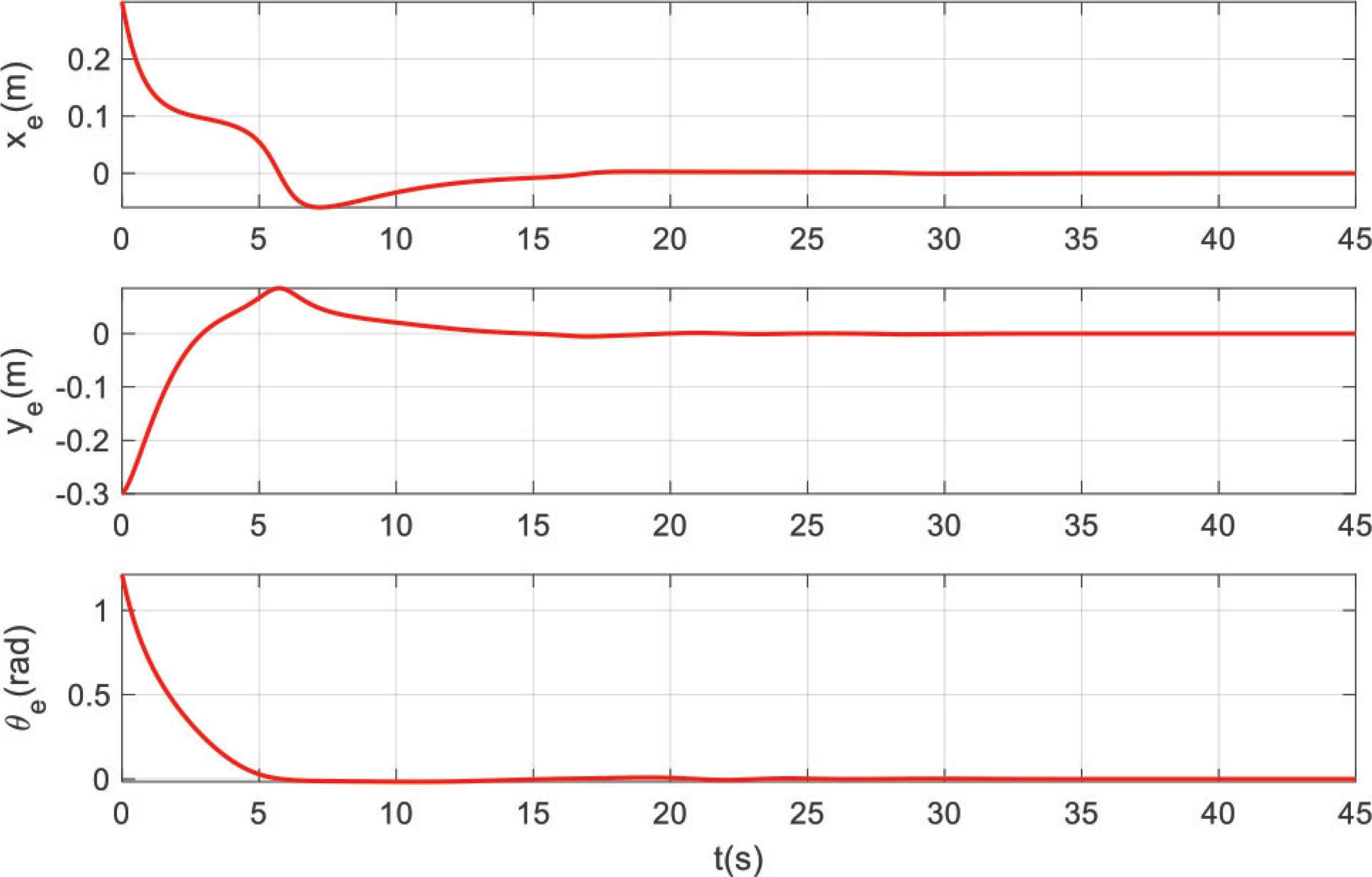
Tracking errors.

Figure 6

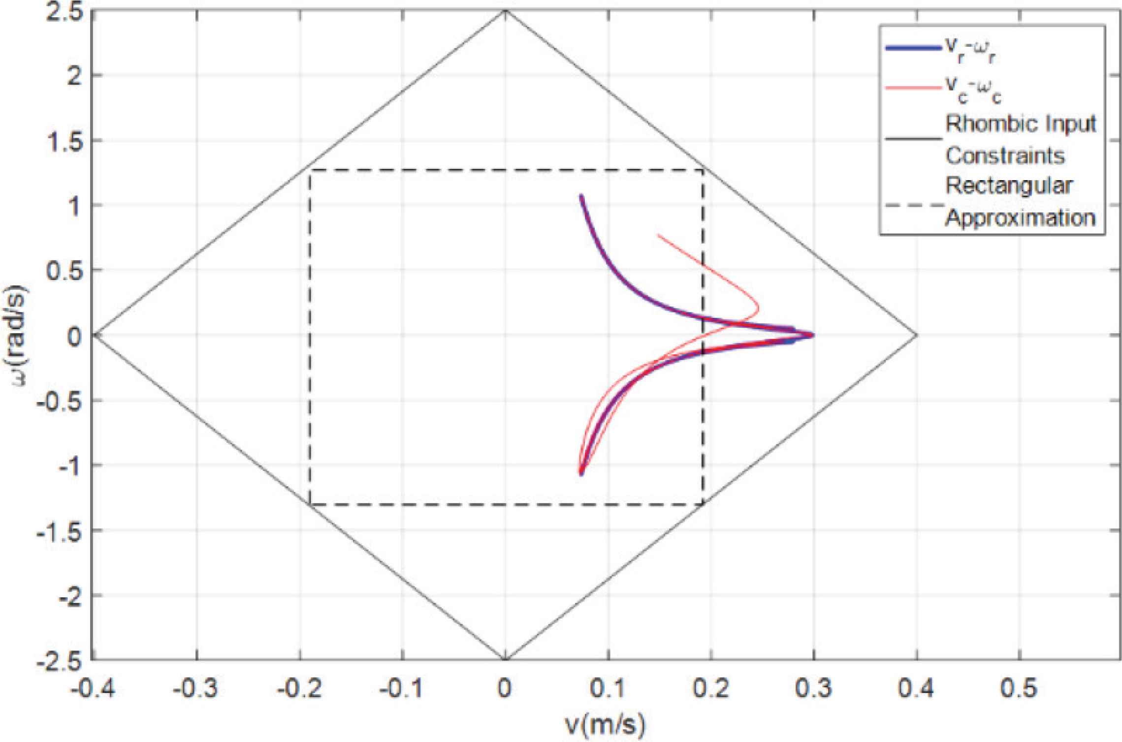
Input and constraints.

Figure 7

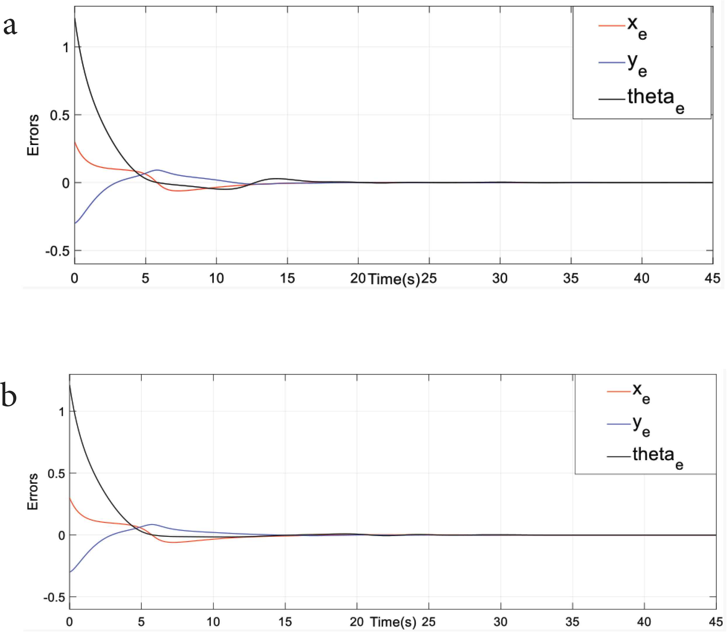
Controller errors comparison.

5. CONCLUSION

The tracking control problem of DWMRs with rhombic input constraints is solved in this paper. Compared with existing methods, we have improved the design of controller parameters and achieved better performance. Also our method can better exert the robots’ mobility and makes the tracking errors converge faster. The controller simultaneously solves the tracking problem and stability problem, its effectiveness can be confirmed by simulation results. Future work will focus on the controller design with uncertainty based on a more complex application environment.

CONFLICTS OF INTEREST

The authors declare they have no conflicts of interest.

ACKNOWLEDGMENTS

This work was supported by the NSFC (62133001, 61520106010) and the National Basic Research Program of China (973 Program: 2012CB 821200, 2012CB821201).

AUTHORS INTRODUCTION

Mr. Kai Gong

He received the B.S. degree in measurement & control technology and instrument from Harbin Engineering University, Harbin, China, in 2016. He is currently pursuing the PhD degree with the Seventh Research Division and the Center for Information and Control, School of Automation Science and Electrical Engineering, Beihang University. His research interests include robotics and motion control.

Prof. Yingmin Jia

He received the B.S. degree in control theory from Shandong University, China, in 1982, and the M.S. and PhD degrees both in control theory and applications from Beihang University, China, in 1990 and 1993, respectively. Then, he joined the Seventh Research Division at Beihang University where he is currently Professor of automatic control. His research interests include robust control, intelligent control and their applications in robot systems.

Mr. Yuxin Jia

He received the B.S. degree in Automation from Chongqing University, Chongqing, China, in 2017. He is currently pursuing the PhD degree with the Seventh Research Division and the Center for Information and Control, School of Automation Science and Electrical Engineering, Beihang University. His research interests include gravity compensation control and intelligent control of mobile robots.