
Design of Nonlinear Internal Model Controller using Local Linear Models, and its Application
- DOI
- 10.2991/jrnal.k.210713.008How to use a DOI?
- Keywords
- Feedback control; local linear models; internal model controller
- Abstract
In chemical plants and other process industries, desired conditions are achieved by adjusting controllers. However, it is difficult to obtain the desired control response because most of the controllers use fixed Proportional-Integral-Differential (PID) control. On the other hand, the internal model control method, in which the control target is described by a detailed mathematical expression, has been proposed. The internal model control is simple to control system structure and is characterized by high robust stability against uncertainties of the control target. However, there are few examples of applying internal model control to nonlinear systems. In this paper, we propose a new method for designing an internal model control system that constructs multiple local linear models for a nonlinear system and adjusts the system parameters corresponding to the models. The effectiveness of the proposed method is verified through experiments.
- Copyright
- © 2021 The Author. Published by Atlantis Press International B.V.
- Open Access
- This is an open access article distributed under the CC BY-NC 4.0 license (http://creativecommons.org/licenses/by-nc/4.0/).
1. INTRODUCTION
In the process industries such as chemical plants, the desired state is achieved by adjusting the controllers. However, most of the controllers use fixed PID control, and it is difficult to obtain the desired control response with a simple controller using fixed parameters when the system has nonlinearity or the system characteristics change significantly due to changes in operating conditions or the environment.
A model-driven control method [1,2] has been proposed in which the control target is described in as detailed a mathematical expression as possible and the model of the control target is incorporated into the control system. One of these model-driven control methods is Internal Model Control (IMC) [3,4]. Internal model control is characterized by the simplicity of the control system structure and its high robust stability against uncertainties of the control target.
For example, a data-driven internal model control system has been proposed, which uses a database to control the system by retrieving data similar to the current data as a neighborhood according to the demand point.
However, these methods require a huge amount of computational time. The authors proposed a method to calculate control parameters using the idea of local linear model method [5]. In this method, multiple local linear models are constructed for a nonlinear system, and the system parameters corresponding to each local linear model are calculated and weighted to design the control system.
In this paper, we propose a method of designing an internal model for a nonlinear system by calculating the system parameters corresponding to each local linear model individually and weighting them. In this method, the system parameters are determined for each local linear model, and the system is expected to be tuned more appropriately for nonlinear systems. Since the database required by the data-driven internal model control system does not need to be constructed, the time required for construction can be reduced. As a result, the load and processing time can be significantly reduced in terms of memory capacity and computation time.
2. IMC DESIGN USING A LOCAL LINEAR MODEL
Local linear models around the equilibrium point are constructed for the nonlinear model according to the characteristics of its static properties. The control parameters corresponding to each local linear model are calculated, and the estimated system output is obtained. Then, the distance between the actual system output and the estimated value is calculated, and the system parameters are load-adjusted according to the distance to achieve nonlinear control. The block diagram of the proposed control system is shown in Figure 1.
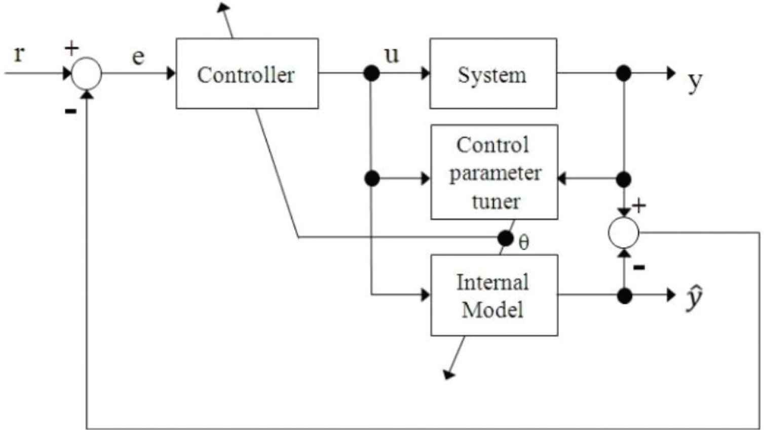
Block diagram of the proposed method.
2.1. System Description
It is assumed that the system dealt with in this paper is given by the following Equation (1).
Furthermore, u(t) is the control input, and ny and nu are the output and input orders, respectively. Now, suppose that the nonlinear system represented by Equation (1) can be locally represented by a linear model like the following Equation (3)
In addition, A(z−1) and B(z−1) are given by the following Equations (4) and (5).
2.2. Designing an Internal Model Controller using a Local Linear Model
In this paper, we consider the control law (IMC) of the following Equations (6) and (7)
In addition, e(t) is a control error signal and can be defined as follows with r(t) as the target value.
Since many real systems have non-linearity, it is difficult to always obtain good control results when the system parameters are fixed. Therefore, in this method, the system parameters included in Equations (4) and (5) are self-adjusted according to the characteristics of the system based on the local linear model, so they are replaced as follows.
After the above preparations, design an internal model controller using a local linear model. The specific algorithm is summarized below.
[STEP 1] Construction of multiple linear models
For the nonlinear model, multiple linear models are constructed, the system is identified by the collective least squares method, and the parameters of A(z−1) and B(z−1) included in the linear model of the following equation are estimated.
[STEP 2] Weight calculation
Next, for each local linear data calculated in [STEP 1], the estimation error ϵi(t); is calculated for each model, and the weight ωi is calculated based on this. ϵi(t); is the error between the system output value y(t); and the estimated output value ỹi(t) of each linear model. Here, ỹi(t) is calculated by the following equation based on Equation (14).
Furthermore, ωi(t) is the weight corresponding to the selected i-th information vector. The smaller the difference between the output value of the actual system and each linear model, the larger this weight becomes. Note that the following equation is satisfied when ωi(t) is calculated based on Equation (19).
[STEP 3] Determining system parameters
Using the weights obtained in [STEP 2] and Ai(z−1) and Bi(z−1) in Equations (15) and (16), the system parameters are calculated by the following Equations (21) and (22).
With this system parameter, Equations (10) and (11) are updated to obtain the output ŷ(t) of the local linear model.
3. EXPERIMENTAL EXAMPLE
The effectiveness of the proposed method will be examined through application to the thermal process system shown in Figure 2. This system uses an incandescent light bulb (40 W) as the control target, and controls the surface temperature of the light bulb by changing the voltage applied to the light bulb by controlling the Joule heat of the filament. A heat transfer pair (R52-CA10AE) sensor is attached to the top of the light bulb. Also, measure the temperature of the light bulb with a thermocouple. Furthermore, the temperature of the thermocouple is converted into a voltage by the thermocouple conversion IC, and after A/D conversion, the data is output to the computer. The control input is calculated using the output data.
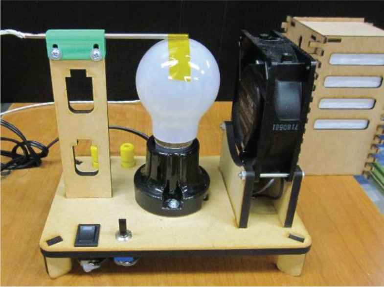
Process system.
A PWM signal with a duty ratio according to the control input is output through D/A conversion, and a current flows through the heater by a Solid State Relay (SSR).
Therefore, the control input u(t) in this experiment is the duty ratio (0–100%) of the PWM signal given to the SSR, and the control output y(t) is the temperature of the surface of the light bulb.
First, the target value r(t) is given as follows.
Next, a local linear model is constructed in the control input range shown below. The number of divisions was N = 2.
Here, the input/output data in the range of u is saved as the initial database. In Equation (24), there is a place where the area of u overlaps, but this avoids that a good response cannot be obtained by selecting the database when the request point is selected near the division of each database. It is provided for this purpose. The values of various design parameters included in the proposed method are ny = 2, ny = 2, and km = 0. Furthermore, the parameters of IMC are λ = 0.5 and n = 1. Here, λ was designed to have the desired rising characteristics.
First, for comparison with the conventional method, the fixed PID control method widely used in the industry is applied. However, for the PID parameter, the value calculated based on the CHR method is used. Its PID parameters are shown below.
First, Figure 3 shows the control results of the fixed PID method and the control results of the proposed method. In addition, Figure 4 shows the temporal change of the weight by the proposed method in this case. From the results in Figures 3 and 4, it can be seen that the weight of the proposed method changes according to the characteristics of the system, and the responsiveness is greatly improved.
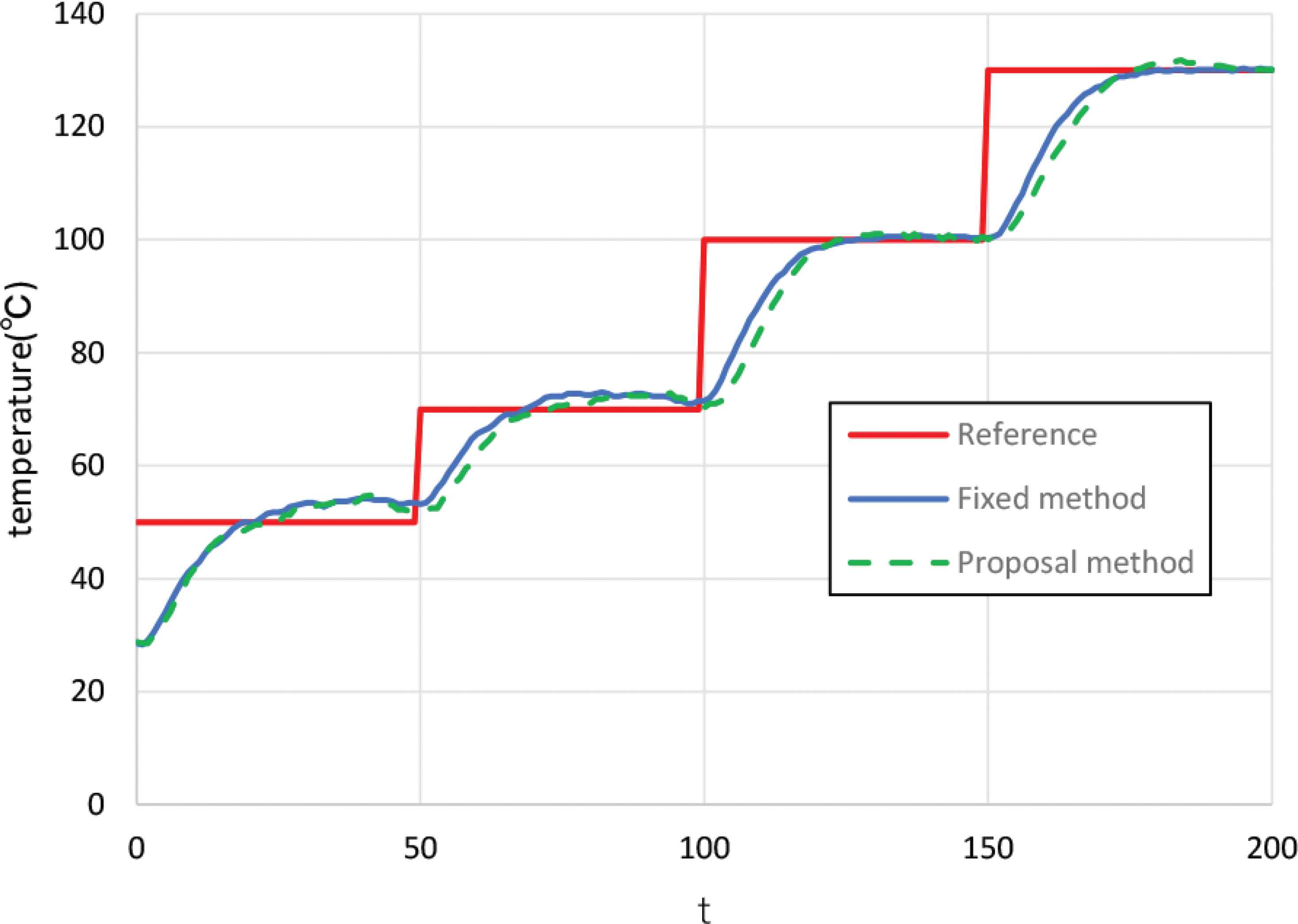
Experimental result.
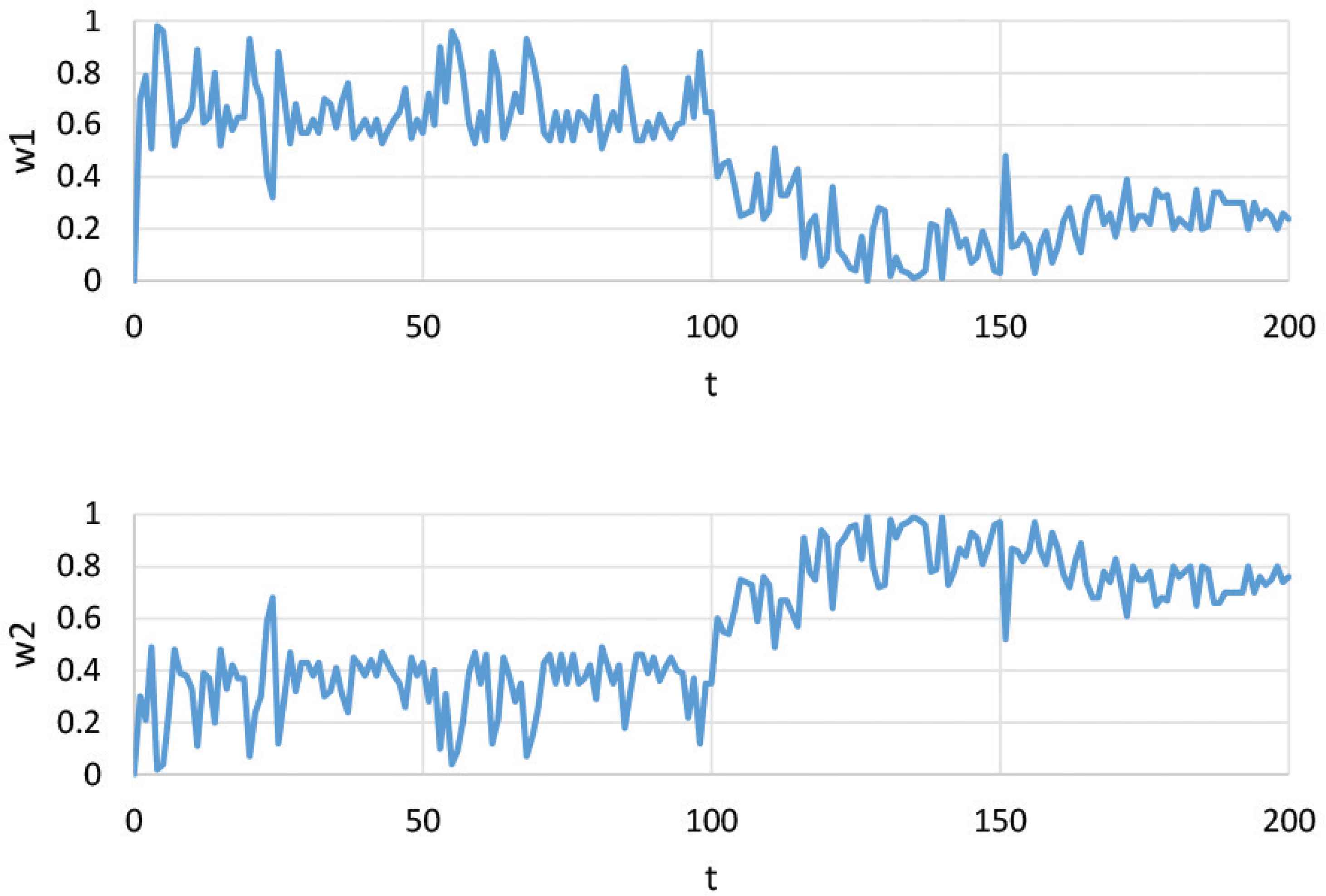
Change in weight.
4. CONCLUSION
In this paper, we have proposed a new method of designing an internal model control system that constructs multiple local linear models for a nonlinear system and adjusts the system parameters corresponding to the models. As a result, it is verified through experiments that the system parameters are appropriately adjusted according to the characteristics of the system and good control results can be obtained. In the future, we plan to study the partitioning method of the local linear model in this method.
CONFLICTS OF INTEREST
The author declares no conflicts of interest.
AUTHOR INTRODUCTION
Dr. Shinichi Imai
 He graduated doctor course at department of engineering in Hiroshima University. He works at department of education in Tokyo Gakugei University. His research area is about control system design, educational engineering.
REFERENCES
Cite this article
TY  - JOUR
AU  - Shinichi Imai
PY  - 2021
DA  - 2021/07/23
TI  - Design of Nonlinear Internal Model Controller using Local Linear Models, and its Application
JO  - Journal of Robotics, Networking and Artificial Life
SP  - 108
EP  - 111
VL  - 8
IS  - 2
SN  - 2352-6386
UR  - https://doi.org/10.2991/jrnal.k.210713.008
DO  - 10.2991/jrnal.k.210713.008
ID  - Imai2021
ER  -