
Novel Mathematical Modeling and Motion Analysis of a Sphere Considering Slipping
- DOI
- 10.2991/jrnal.k.190531.006How to use a DOI?
- Keywords
- Angular velocity vector of the sphere; motion analysis of the sphere; slip velocity of the sphere
- Abstract
Many mobile robots that use spherical locomotion employ friction-drive systems because such systems offer omnidirectional locomotion and are more capable of climbing steps than omni-wheel systems. One notable issue associated with friction-drive systems is slipping between the sphere and the roller. However, previously established sphere kinematics models do not consider slipping. This study proposes a mathematical model that allows for slipping and can be broadly applied to a variety of mobile robots in a range of situations.
- Copyright
- © 2019 The Authors. Published by Atlantis Press SARL.
- Open Access
- This is an open access article distributed under the CC BY-NC 4.0 license (http://creativecommons.org/licenses/by-nc/4.0/).
1. INTRODUCTION
Spherical wheels can be used in mobile and omnidirectional robots. For example, the ball wheel [1] comprises a sphere with a circular-roller ring arranged on the outer circumference of the sphere. The propulsive force is generated by the rotation of the oblique-rotation axis. Further, there is no binding force in the direction orthogonal to the propulsion force as there is with an omni-wheel [2]. The omni-ball [3] solves the constraint of the ball wheel [1] as it enables omnidirectional driving via the passive rotation of a pair of hemispheres. It offers similar driving performance as the omni-wheel [2] and superior step-climbing ability.
In mobile robots, Active-Caster [4] is composed of an upper sphere and a lower sphere, each of which is in contact with two driving rollers. The upper sphere uses driving rollers to transmit dynamic motion to the lower sphere. This mechanism is used for driving and steering of the caster and enables omnidirectional motion. The balanced-ball robot [5] achieves omnidirectional locomotion by spherical driving using three omni-wheel arranged on the upper hemisphere of an equilateral triangle. The CPU-ball robot [6] has four-omni-wheel arranged on the upper hemisphere of a regular quadrilateral to achieve spherical driving and realize omnidirectional locomotion.
The RoboCup middle-size-league soccer robot utilizes a ball-dribbling mechanism to control the rotation of the ball. Most of the RoboCup teams, such as the Turtles [7], implemented two constraint rollers on the upper half of the ball. Due to makes strong friction force and enhanced ball-holding ability, most designs use slip-roller arrangements as are determined heuristically via experiments in the absence of suitable mathematical models.
In a previous study, we developed a non-slip omnidirectional-locomotion kinematics model that accounts for the sphere kinematics and roller arrangement [8]. However, this model cannot be used for mobile robots as they also undergo slip locomotion. In this study, we modify the previously developed kinematics model and present a novel mathematical model of sphere rotational motion by two constraint rollers that allows for slipping.
In this paper, the outline of the section is as follows: Section 2 consider discusses the existence space of angular velocity vector and the sphere kinematics by two roller. Section 3 conducted simulation. Finally, we present the summary and discuss future tasks.
2. THE SPHERE KINEMATICS BY CONSTRAINT ROLLERS
In this section, we introduce the angular velocity vector of the sphere to algebraically model the sphere rotational motion.
2.1. The Existence of Angular Velocity Vector of the Sphere by Single-constraint Roller
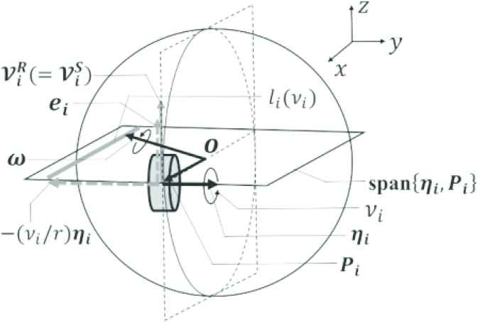
As shown in Figure 1, the center O of a sphere with radius r is fixed as the origin of the coordinate system Σ − xyz. Table 1 shows the variables related to the sphere kinematics. The ith constraint roller is in point contact with the sphere at a position vector Pi and is arranged such that the center of mass of the roller Pi and O are on the same line. ω denotes the angular velocity vector of the sphere. ηi denotes the unit vector along the rotational axis of constraint roller. νi denotes the peripheral speed of the constraint roller. Hence, the velocity vector of the sphere
The existence of sphere angular velocity vector in case of single-constraint roller.
| Σ−xyz | Three-dimensional coordinate system fixed the sphere |
| 〈a, b〉 | Inner product with respect to a and b |
| ‖a‖ | Norm of vector a |
| span{X, Y} | The existence space of ω allow for slip |
| O | The sphere center |
| Pi | The Position vector of sphere |
| ηi | The unit vector along the rotational axis of the constraint-roller |
| ω | The angular velocity vector of the sphere |
| ωt | The orthogonal projection of ω with respect to span{P1, P2} |
| ωs | The orthogonal projection of ω with respect to P1 × P2 |
|
|
The velocity vector of constraint roller |
|
|
The velocity vector of the sphere |
| ζi | Slip velocity of the sphere with respect to
|
| ei | The unit normal vector along
|
| e | Upper unit normal vector of span{P1, P2} |
| V | Mobile velocity of sphere on xy-plane |
| {Xi, e} | Normal orthogonal bases on tangent plane of the sphere at Pi |
| li(νi) | Set that exists of end point of ω |
| The orthogonal projection of li(νi) with respect to span{P1, P2} | |
| νi | Peripheral speed of constraint roller |
| r | The sphere radius |
| αi | The roller arrangement angle between ηi and span{P1, P2} |
| φ | Sphere direction |
| ρ | Angle of sphere rotational axis |
The variables related to the sphere kinematics
Thus, ω can be satisfied as Equation (3).
Further, from the property of the constraint roller (i.e., that slip does not occur in side direction of the roller), ω must be on span{ηi, Pi}. Thus, Eq. (3) indicates that ω is constructed as the sum of (νi/r)ηi and Pi (see Figure 1). Thus, ω cannot be uniquely determined using a single roller. However, the end point set of ω can be represented as a line set as follows:
2.2. The Existence of Angular Velocity Vector of the Sphere by Two-constraint Rollers
Let the roller arrangement the angle αi (−90° ≤ αi ≤ 90°) between ηi and span{P1, P2}. Using the normal orthogonal base {Xi, e} on tangent plane of the sphere at Pi, ηi can be represented as Equation (5).
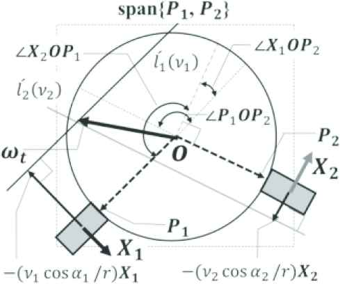
In this section, we consider location between l1(ν1) and l2(ν2) which depend on parameter ν1, ν2 (when α1, α2 are fixed) and determined the rotational axis of the sphere.
Using Equation (4) (as i = 1, 2), as shown in Figure 2a, if a pair of ν1, ν2 exists such that l1(ν1) and l2(ν2) have points in common, the end point of ω can be uniquely determined. Using Equation (4) (as i = 1, 2), ω must be on span{P1, η1}∩span{P2, η2}. On the other hand, as shown in Figure 2b, if a pair of ν1, ν2 exists such that l1(ν1) and l2(ν2) have no points in common, slip can occur.
Because the sphere rotational axis is defined with respect to the arbitrary parameters ν1 and ν2, Qo ∈ ℝ3 can be determined such that the sum of the squared distances between Q ∈ ℝ3 and li(νi) (i = 1, 2) is minimized. Then, Qo corresponds to the mid-point between l1(ν1) and l2(ν2) [see Appendix (A)]. Using Xi, Pi, orthogonal projection of li(νi) with respect to span{P1, P2} is represented as Equation (7).
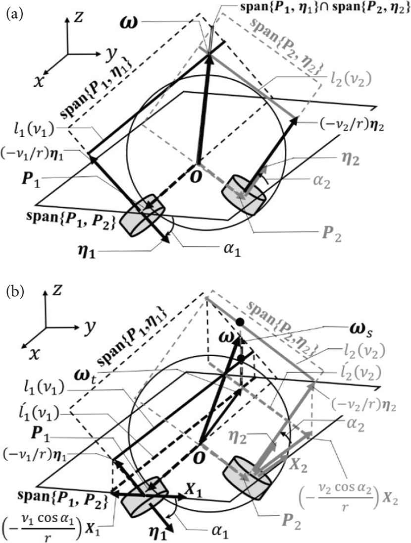
The location of l1(ν1) and l2(ν2). (a) A pair of ν1, ν2 exists such that l1(ν1) and l2(ν2) have points in common. (b) A pair of ν1, ν2 exists such that l1(ν1) and l2(ν2) have no points in common.
The end point of ωt (the orthogonal projection of ω with respect to span{P1, P2}) is represented as common point of
A heights li(νi) from span{P1, P2} (i = 1, 2), is represented as follows:
Using Equation (9), ωs (the orthogonal projection of ω with respect to P1 × P2) is represented as mean of these.
Thus, ω can be represented with respect to ν1 and ν2 ∈ ℝ.
Specifically, when αi = 0°, the second term of the right-hand side of Equation (11) vanishes. Thus, for all ν1, ν2, ω ∈ span{P1, P2}. In other words, the sphere has omnidirectional locomotion without slip in the expanded form of kinematics model [8].
2.3. The Sphere Kinematics by Two-constraint Rollers
2.3.1. Forward kinematics
φ (0° ≤ φ < 360°) is the angle from x-axis. Mobile velocity of sphere V (the center velocity of sphere) is on xy-plane and represented as Equation (13).
2.3.2 Inverse kinematics
From Equations (13) and (14), ω is represented as Equation (15).
By rearranging Equation (11), following equation can be obtained as linear combination of X and Y.
Thus, for all ν1, ν2, span{X, Y} is two-dimensional-freedom existence space, which has the unit vector X × Y. From ω ∈ span{X, Y}, using Equation (15) and 〈ω, X × Y〉 = 0, ρ is obtained as follows:
When Equation (18) is substituted in Equation (15), ω is obtained as follows:
And, from Equation (7), ω is satisfied as
Using Equation (6), 〈ω, Xi〉 is calculated as follows:
Thus, from Equations (20) and (21), νi is obtained as follows:
2.4. Slip Velocity of the Sphere
Slip occurs when the roller velocity
Here, we substitute (24) for
Taking the inner product with e on both sides of Equation (25) and using Equation (22) in the first term on the right-side and Equation (5) in the second term of the right-side, the following Equation (26) can be formulated.
Thus, ζi is parallel to Xi (e-component vanished) and represented as
3. SIMULATION
This section presents the simulation results, including the trajectory of the end point of the angular velocity vector, the angle of the sphere rotational axis, the peripheral speed of the constraint roller, and Xi-component of the slip velocity in the given mobile speed of the sphere: ||V||=1 m/s. The conditions are as follows: r = 1 (m), θ1,1 = 215°, θ1,2 = 325°, θ2,2 = 60°, and α2 = −α1. Simulations were conducted at the four different angles, α1 [represented as k; curve color]. Further, ωk, ρk, νi,k, and Si,k (k = 0, 1, 2, 3) were indicated such as α1 = 0° [k = 0; red curve], α1 = 10° [k = 1; blue curve], α1 = 20° [k = 2; green curve], and α1 = 30° [k = 3; pink curve]. They are calculated from Equations (18), (19), (22), and (28), respectively. As shown in Figure 3a, ellipsoid trajectories ωk (k = 0, 1, 2, 3) are getting scarp in turn and have a common line parallel to the x-axis.
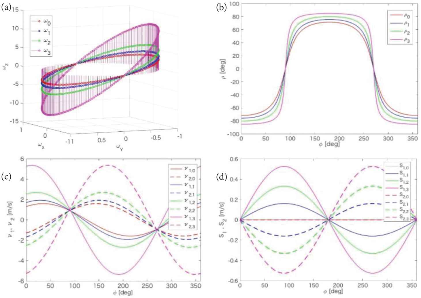
Comparison in case of α1 = 0°, 10°, 20°, 30° in simulation. (a) Trajectory of end point of angular velocity vector of the sphere. (b) Angle of the sphere rotational axis. (c) Rollers peripheral speed. (d) Xi-component of slip velocity of the sphere.
As shown in Figure 3b, ρk (k = 0, 1, 2, 3) satisfy the inequality |ρ0| < |ρ1| < |ρ2| < |ρ3| for all φ. Specifically, when φ = 90° or 270°, ρk = 0°. Thus, the sphere undergoes pure rotation (forward and backward movement).
As shown in Figure 3c, νi,k (k = 0, 1, 2, 3) are satisfied |νi,0| < |νi,1| < |νi,2| < |νi,3| (i = 1, 2) For all φ. Specifically, where φ = 0° and 180° (right and left side forward movement), ν1,k = −ν2,k (opposite sign). Where φ = 90° and 270°, ν1,k = ν2,k and |νi,0| = 0.91, |νi,1| = 0.93, |νi,2| = 0.96, |νi,3| = 1.03 (m/s).
As shown in Figure 3d, Si,k (k = 0, 1, 2, 3) satisfy the inequality |Si,0| < |Si,1| < |Si,2| < |Si,3| (i = 1, 2) for all φ. From Equation (26), where 0° < φ < 180°, ζ1,k and ζ2,k are face-to-face. In contrast, where 180° < φ < 360°, ζ1,k and ζ2,k are back-to-back. Specifically, when φ = 0° and 180°, the sphere slip speed is ||ζ1,k||=||ζ2,k||=0 m/s. Specifically, when φ = 90° and 270°, |S1,k| and |S2,k| are at their maxima (|S1,0|=|S2,0|=0, |S1,1|=|S2,1|=0.16, |S1,2|=|S2,2|=0.32, and |S1,3|=|S2,3|=0.52 m/s).
Further, when α1 = 0°, |S1,0|=|S2,0|=0 for all φ. Thus, in this case, the sphere has omnidirectional locomotion without slip. Moreover, the proposed model includes the previously developed model [8].
4. CONCLUSION
Herein, we consider the existence of an angular velocity vector for the sphere and propose a sphere kinematics model that allows for slipping. In addition, we demonstrate the trajectory of the end point of the angular velocity vectors of the roller speed and slip speed of the sphere in simulations. This model includes the previously developed model [8] and is expected to be applicable to a wide range of mobile robots in a variety of situations.
In future studies, this model should be verified experimentally. Further, it could be applied to simulate the ball-dribbling mechanism.
CONFLICTS OF INTEREST
There is no conflicts of interest.
APPENDIX (A) CALCULATION OF MINIMAL POINT Q0
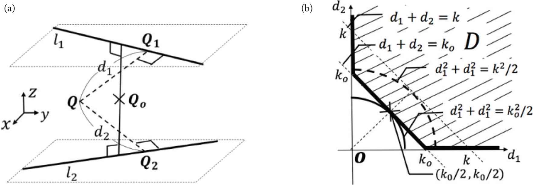
As shown in Figure 4a, di denote the distance between Q ∈ ℝ3 and line li (i = 1, 2). Qi denote the points at which a perpendicular line intersects li (i = 1, 2). Using follow
Lemma.
Let k0 be the minimum value of d1 + d2 and Mk = {X|d1 + d2 = k, k0 ≤ k, k ∈ ℝ, X ∈ ℝ3}.
The following statements hold:
- (i)
- (ii)
Minimum problem of sum of squares distance. (a) Problem (A): Minimum
Problem (A): Minimum of
Thus, as shown in Figure 4b, when the line defined by d1 + d2 = k0 is tangent to the circle defined by
APPENDIX (B) CALCULATION OF ωt
As shown in Figure 5, following expressions are completed.
The end point of ωt on span{P1, P2} is determine as common point
Using Equations (B.1) and (B.3), 〈P2, X1〉 are represented as Equation (B.4).
Using Equations (B.2) and (B.4), 〈P1, X2〉 are represented as Equation (B.5).
ωt can be represented as shown in Equation (B.6).
In both the sides of Equation (B.6), taking inner product with respect to Xi. 〈ωt, Xi〉 is represented as Equation (B.7).
Using Equation (20), ωt is satisfied Equation (B.8).
Using 〈Pi, Xi〉 = 0 and Equation (B.8), right side of Equation (B.7) is represented as Equation (B.9).
Thus, using Equation (B.5), C1 and C2 are represented as Equation (B.10).
Equation (B.10) is substituted in Equation (B.6). Thus, it is given.
Authors Introduction
Mr. Kenji Kimura
 He received the M.E. (mathematics) from Kyusyu University in 2002. Then he was a mathematical teacher and involved in career guidance in high school up to 2014. He currently, is instructor of International Baccalaureate Diploma Program (Mathematics: applications and interpretation, analysis and approaches) in Fukuoka Daiichi High School, and student in the doctoral program of the Kyushu Institute of Technology. His current research interest spherical mobile robot kinematics, control for object manipulation, and human body motion Bernstein’s degrees-of freedom problem.
Mr. Kouki Ogata
 He received high school diploma in Fukuoka Daiichi high school until 2016. He is currently under Graduate School student at Saga University. His current research interest sphere mobile robot kinematics, control, analytical dynamics.
Dr. Kazuo Ishii
 He is a Professor in the Kyushu Institute of Technology, where he has been since 1996. He received his PhD degree in engineering from University of Tokyo, Tokyo, Japan, in 1996. His research interests span both ship marine engineering and Intelligent Mechanics. He holds five patents derived from his research. His lab got “Robo Cup 2011 Middle Size League Technical Challenge 1st Place” in 2011. He is a member of the Institute of Electrical and Electronics Engineers, the Japan Society of Mechanical Engineers, Robotics Society of Japan, the Society of Instrument and Control Engineers and so on.
REFERENCES
Cite this article
TY  - JOUR
AU  - Kenji Kimura
AU  - Kouki Ogata
AU  - Kazuo Ishii
PY  - 2019
DA  - 2019/06/17
TI  - Novel Mathematical Modeling and Motion Analysis of a Sphere Considering Slipping
JO  - Journal of Robotics, Networking and Artificial Life
SP  - 27
EP  - 32
VL  - 6
IS  - 1
SN  - 2352-6386
UR  - https://doi.org/10.2991/jrnal.k.190531.006
DO  - 10.2991/jrnal.k.190531.006
ID  - Kimura2019
ER  -