
Kernel Density Estimation of White Noise for Non-diversifiable Risk in Decision Making
- DOI
- 10.2991/jracr.k.200421.003How to use a DOI?
- Keywords
- Curve estimation; non-diversifiable risk; random variable; probability estimates
- Abstract
Many businesses make profit yearly and tend to invest some of the profit so that they can cushion their organizations against any future unknown events that can affect their current profit making. Since future happenings in businesses cannot be predicted accurately, estimates are made using experience or past data which are not exact. The probability element (which is normally determined by experience or past data) is important in investment decision making process since it helps address the problem of uncertainty. Many of the investment decision making methods have incorporated the expectation and risk of an event in making investment decisions. Most of those that use risk account for diversifiable risk (non-systematic risk) only thus limiting the predictability element of these investment methods since total risk are not properly accounted for. A few of these methods include the certainty (probability) element. These include value at risk method which uses covariance matrices as total risk and the binning system which always assumes normal distribution and thus does not take care of discrete cases. Moreover comparison among various entities lacks since the probabilities derived are for individual entities and are just quantile values. Finite investment decision making using real market risk (non-diversifiable risk) was undertaken in this study. Non-diversifiable risk (systematic risk) estimates of a portfolio of stocks determined by a real risk weighted pricing model are used as initial data. The variance of non-diversifiable risk is estimated as a random variable referred to as random error (white noise). The estimator is used to calculate estimates of white noise (wn). A curve estimation of the wn is made using Kernel Density Estimation (KDE). KDE is a non-parametric way to estimate the probability density function of a random variable. KDE is a fundamental data smoothing problem where inferences about the population are made, based on a finite data sample. This is used to derive probability estimates of the non-diversifiable risks of the various stocks. This enables determination of total risk with given probabilities of its occurrence thus facilitating decision making under risky and uncertain situations as well as accentuating comparison among the portfolio of stocks.
- Copyright
- © 2020 The Authors. Published by Atlantis Press SARL.
- Open Access
- This is an open access article distributed under the CC BY-NC 4.0 license (http://creativecommons.org/licenses/by-nc/4.0/).
1. INTRODUCTION
In the past few years there has been evidence of collapse of well-established business entities. This has been attributed to lack of accurate methods of preventing or measuring risk and uncertainty as opposed to lack of the same methods. Many companies on Wall Street in 2008 went under despite having extensive measures of mitigating risk such as futures and forward. An investigation into some of these methods reveals the lack of a well-estimated market risk measure in the models. It is an obvious fact now that it was the external reactions that brought down the companies on Wall Street. Once the markets got a hint of the internal financial and investment affairs of the companies this spread so rapidly and in a matter of hours these companies had collapsed. A good example is the Lehman Brothers Holdings limited, Merrill Lynch and companies, and American Investment group as explained by Lucchetti et al. [1]. These indicate that market environments are so critical in the existence of business entities such that variables affecting the business entities from the market environments should be estimated with a lot of precision. This paper determines total risk which has both the systematic and non-systematic components. It should be noted that the non-systematic risk is internal in nature, and in most cases well known and relatively less difficult to estimate while systematic is external and in most cases is embodied in market risk.
This paper will determine the risk factor of systematic risk a phenomenon lacking in many risk models. Since we have seen from most examples that market risk is the precursor of most companies down falls, it is hoped that investors and companies will be able to easily estimate riskiness of the risk measures thus enabling them make informed decisions.
Jorion [2] determines the Value at Risk (VAR) measure as the forecasted volatility, St multiplied by standard normal deviate, α for the selected confidence level (e.g. α = 2.33 for a one-tailed confidence level of 99%). The portfolio variance then becomes
Dennis et al. [3] in estimating density dependence process noise and observation error offers a statistical approach for jointly estimating density dependence, process error and observation error. Although this model is relatively easy for ecologists to use and is applicable in many population systems, this process noise has a normal distribution with mean μ and variance σ2 (Et ∼ N(0, σ2)). This paper looks at a case of no assumption of normality for the noise process. White noise is determined as a random variable on the precincts of Sklar [4] where he says no common probability space can be found for a given set of random variables, but such common probability spaces exists for arbitrary proper subsets of the given set. In this study the subsets were the portfolios of different companies used giving a common probability space that is estimated. The results of Wu [5] show that for finite parameters the consistency of the least squares estimator is equivalent to the existence of a consistent estimator thus the estimator of white noise derived in this paper is an unbiased estimator.
2. RISK OF NON-DIVERSIFIABLE RISK
2.1. Determination of White Noise of Non-diversifiable Risk
White noise refers to a purely random process whose random variables are a sequence of mutually independent, identically distributed random variables. Thus it describes an event and is a function with a domain that makes some real number correspond to each outcome of the experiment. In this paper white noise is taken as the random error of non-diversifiable risk NGwi of an investment i. To add credence to this study it is imperative to show that white noise is a random variable. Proposition 2.1 below seeks to do so.
Proposition 2.1:
Let Vi be the white noise of the non-diversifiable risk NGwi, then Vi(.) is a random variable.
Proof: Given NGwi and
- i.
The domain Ω
- ii.
The counter domain r is such that 0 ≤ r ≤ 1.
- iii.
The range of returns i is −∞ ≤ i ≤ ∞.
Then the probability of Vi(.), P[Vi(.)] is a set function having domain Vi(.) and counter domain the interval [0,1]. Therefore Vi(.) has a probability space (Ω, W, P[Vi(.)]). Also W consists of four subsets;
Such that if:
- i.
r < 0, then s:Vi(s) ≤ r = ϕ.
- ii.
0 ≤ r < 1, then s:Vi(s) ≤ r, where
- iii.
r ≥ 1, then {s:Vi(s) ≤ r} = Ω =
Since Vi(.) has a probability space, and W consists of the four subsets above. Then for each r the set {s:Vi(s) ≤ r} belongs to W, thus Vi(.) is a random variable. Since Vi(.) is a random variable and it is independent with unique parameters. Therefore the parameters of white noise for example its mean and variance as well as its unique probability distribution can be determined. The probability estimates of non-diversifiable risk for investment decisions are then estimated as shown in the following subsections.
2.1.1. Determination of random error
The non-diversifiable variance estimator
From (2) the actual value of
Let the variance between actual and sample white noise be
The values of C and L which will minimize variance are given by the partial derivatives of C and L, fC and fL respectively. After several iterations;
Thus the value of
Proposition 2.2:
Proof: From Equation (2)
Dividing Equation (6) by z results in
Thus
From the results of Wu [7], Equation (6) and proposition 2.2,
3. DERIVATION OF A PROBABILITY DENSITY FUNCTION FOR RANDOM ERROR OF NON-DIVERSIFIABLE RISK
3.1. Kernel Density Estimation of White Noise of Non-diversifiable Risk
Let V1,V2,...,Vn denote a sample of size n from the random variable Vi(.) with density f. The kernel density estimates of f at the point v is given by
Proposition 3.1:
Proof:
Given the function
since,
Let
Then
Meaning that it is independent of
It is generally known that the value of the bandwidth is of critical importance while the shape of the kernel function has little practical impact. Thus we estimate bandwidth and use a given kernel function to get the density estimation of the white noise of non-diversifiable risk.
3.2. Bandwidth Selection for Kernel Density Estimation of the wn of Non-diversifiable Risk
Assuming that the underlying density is sufficiently smooth and that the kernel has fourth moment using the Taylor series
The overall measure of the discrepancy between
Under an integrability assumption on f, integrating the expression for AMSE gives the expression for the Asymptotic MISE (AMISE), i.e.,
The value of the bandwidth that minimizes the AMISE is given by
Using the rule of thumb method a global bandwidth h is based on replacing R(f″) the unknown part of hAMISE, by its value for a parametric family expressed as a multiple of a scale parameter, which is then estimated from the data. The method dates back to Deheuvels [10] and Scott [11]. It has been popularized for kernel estimates by Silverman [12].
The plug-in method is used to estimate hAMISE in this study. Here the unknown quantity R(f″) in the expression for hAMISE is replaced by an estimate. The “solve - the - equation” plug-in approach developed by Sheather and Jones [13] is based on deriving, the pilot bandwidth for the estimate R(f″), as a function of h, namely
The unknown functions of f are estimated using kernel density estimates with bandwidth based on normal rules of thumb resulting in
The triangle kernel is used for smoothing
This is given by
This function is used to generate probabilities of non-diversifiable risks of given portfolio thus ensuring that actual systematic risk is determined.
4. RESULTS
4.1. Calculating Actual Non-diversifiable Risk
The sample white noise is estimated by varying the variance of individual return values ri as given by Equation (2). The non-diversifiable risk estimates in Table 1 are substituted into Equation (3) to give Equation (5).
| Company | σn |
|---|---|
| YH | 29.33 |
| TIF | 63.5 |
| TM | 538.1 |
| HM | 28.23 |
| PONARD | 27.97 |
| VIC | 0.561 |
| DAWT | 25.58 |
| BP | 105.2 |
| SUNTB | 108.3 |
| PNC | 7.876 |
| AIG | 7164 |
| FORD | 1898 |
| AMR | 25.17 |
| BPH | 1.752 |
| CTL | 5.547 |
| PFE | 46.58 |
| RTI | 9.054 |
| GSK | 35.81 |
The non-diversifiable risks of 20 stocks from NYSE
Sample wn estimates are then substituted into Equation (5) to determine the actual white noise.
4.2. Density Estimates of Actual White Noise
R statistical software is used to calculate Sheather–Jones (sj) bandwidth and hence the density estimates of actual wn as plotted in Figure 1.
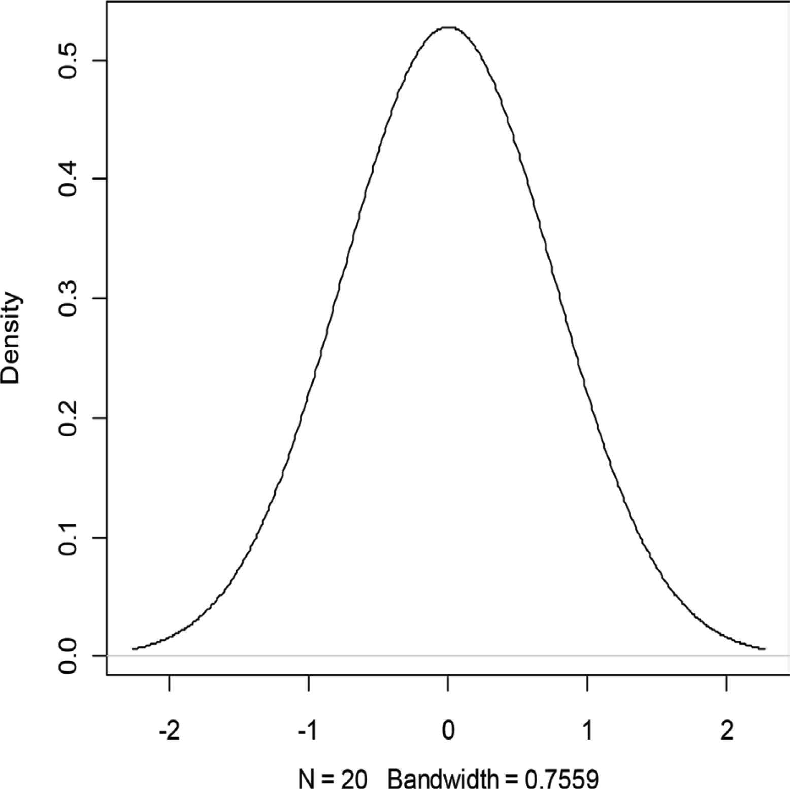
A plot of the density estimates of actual white noise. Call: Density (x = x, bw = 0.7559, x lim = c(−2, 2)). Data: x (20 obs.); Bandwidth “bw” = 0.7559.
A summary of statistics resulting from sj density estimation in Table 2 enables us apportion densities of the different quartile ranges.
| Company | wn | F | Probabilities | Actual σn |
|---|---|---|---|---|
| YH | 0.000729 | 0.827722 | 0.63566 | 18.64391 |
| TIF | 0.00027 | −0.27869 | 0.491 | 31.1785 |
| TM | 0.00011 | −0.66196 | 0.4414 | 237.5173 |
| HM | 0.000128 | −0.62098 | 0.4467 | 12.61034 |
| PONARD | 0.001551 | 2.809139 | 0.979 | 27.38263 |
| VIC | 0.00046 | 0.179302 | 0.5511 | 0.309222 |
| DAWT | 0.001456 | 2.580143 | 0.9388 | 24.0145 |
| BP | 0.000113 | −0.65714 | 0.442 | 46.4984 |
| SUNTB | 0.00011 | −0.66437 | 0.441 | 47.7603 |
| PNC | 0.000142 | −0.58723 | 0.4511 | 3.552864 |
| AIG | 0.000657 | 0.654167 | 0.613 | 4390.919 |
| FORD | 0.000308 | −0.18709 | 0.5033 | 954.7601 |
| AMR | 0.000491 | 0.254027 | 0.521 | 13.11357 |
| BPH | 0.000227 | −0.38234 | 0.4778 | 0.837106 |
| CTL | 0.0000884 | −0.71655 | 0.4342 | 2.408507 |
| PFE | 0.0000988 | −0.69146 | 0.4375 | 20.37875 |
| RTI | 0.000238 | −0.35582 | 0.4813 | 4.35769 |
| GSK | 0.0000872 | −0.71933 | 0.4339 | 15.53796 |
| BCE | 0.00022 | −0.39921 | 0.4756 | 99.44796 |
| STGI | 0.000227 | −0.38234 | 0.4778 | 7.601798 |
Final results of white noise and kernel density estimation of portfolios of stocks
F-values are calculated as follows:
Final results of the survey are tabulated in Table 3.
| X | Y |
|---|---|
| Min.:−2.2676128 | Min.: 0.005892 |
| 1st Qu.: 1.133396 | 1st Qu.: 0.041992 |
| Median: 0.00081 | Median: 0.170879 |
| Mean: 0.0008191 | Mean: 0.219614 |
| 3rd Qu.: 1.135035 | 3rd Qu.: 0.397272 |
| Max.: 2.269251 | Max.: 0.527674 |
A summary of the results of a kernel density estimation of a portfolio white noise
4.3. Wilcoxon Signed Rank Test
Wilcoxon signed rank test of hypothesis is used to compare the VaR method of determining risk and Kernel white noise method.
Here we test the hypothesis that risks obtained by Kernel white noise are a reflection of actual risks than those obtained by VaR.
Ho: The population difference are centered at 0.
Ha: The population differences are centered at a value <0.
Based on a significance level of α = 0.01, the proper test is to reject Ho if Z < −Zα. Determining Z and
Using normal tables −Zα = −1.645, using the difference in risks and their ranks in Table 4 (Z = −3.88).
| Company | Actual σn(i) | VaR at α = 0.01 (ii) | (i) – (ii) | Rank |
|---|---|---|---|---|
| Yahoo | 18.64 | 0.4699 | 18.17 | 10 |
| Tiffany | 31.18 | 0.2693 | 30.91 | 14 |
| Toyota | 237.52 | 0.1790 | 237.34 | 18 |
| HM | 12.61 | 0.1688 | 12.44 | 7 |
| Ponardph | 27.38 | 0.8349 | 26.55 | 13 |
| Vical Inc | 0.31 | 0.4629 | −0.15 | 1 |
| Data Watch | 24.01 | 0.8398 | 23.17 | 12 |
| Bp | 46.50 | 0.1391 | 46.36 | 15 |
| Suntrust | 47.76 | 0.2145 | 47.55 | 16 |
| Pnc | 3.55 | 0.1914 | 3.36 | 4 |
| AIG | 4390.92 | 0.5951 | 4390.32 | 20 |
| Ford | 954.76 | 0.3662 | 954.39 | 19 |
| Amr | 13.11 | 0.4806 | 12.63 | 8 |
| Bph | 0.84 | 0.2036 | 0.63 | 2 |
| Ctl | 2.41 | 0.1978 | 2.211 | 3 |
| Pfe | 20.38 | 0.1607 | 20.22 | 11 |
| Rti | 4.358 | 0.3184 | 4.039 | 5 |
| Gsk | 15.54 | 0.1297 | 15.41 | 9 |
| Bce | 99.45 | 0.1775 | 99.27 | 17 |
| Sbg | 7.602 | 0.3714 | 7.230 | 6 |
A table of Wilcoxon signed rank test for large samples paired
Since, Z < Zα we reject the null hypothesis, so there is sufficient evidence to conclude that the kernel white noise risks are a reflection of actual risks as compared with those obtained by VaR.
5. CONCLUSION
An estimate of random error is made with the least bias and variance. Probability estimates of the asset parameters are made thus boosting the level of surety. These are made in comparison i.e. looking at given portfolios one is able to make a decision among a variety of them. Methods like VaR use generated variances to give probability estimates using extreme values. This lacks the comparability factor and assumes the central limit theory leading to application of normality conditions. They also use covariance parameters as market risks thus going against its definition. A case study of New York Stock Exchange (NYSE) Dow index in 2008 indicates that the portfolios with the highest actual non-diversifiable risks were AIG with 4390.919%, FORD; 954.7661%, and TM; 237.5173%. These are corporates which experienced financial difficulties during the credit crunch in the USA in 2008. AIG and TM had to be given some financial rescue packages to stay afloat until the financial crump was reversed. From the analysis of the results from the NYSE case study of the Dow index in 2008 it is clear that there is a relationship between the determined actual non-diversifiable and the actual market risk on the ground over the past 2 years. These research findings can aid investors make solid investment decisions as well as the different corporate cut ion themselves against any financial stress currently and in future.
CONFLICTS OF INTEREST
The authors declare they have no conflicts of interest.
AUTHORS’ CONTRIBUTION
The original idea and subsequent analysis of the research was undertaken by EAS with the guidance of PW and TA.
ACKNOWLEDGMENTS
I wish to acknowledge the University of Nairobi staff in the school of Mathematics as well as my family members for their encouragement and support during the period of undertaking this research.
REFERENCES
Cite this article
TY  - JOUR
AU  - Emma Anyika Shileche
AU  - Patrick Weke
AU  - Thomas Achia
PY  - 2020
DA  - 2020/04/27
TI  - Kernel Density Estimation of White Noise for Non-diversifiable Risk in Decision Making
JO  - Journal of Risk Analysis and Crisis Response
SP  - 6
EP  - 11
VL  - 10
IS  - 1
SN  - 2210-8505
UR  - https://doi.org/10.2991/jracr.k.200421.003
DO  - 10.2991/jracr.k.200421.003
ID  - Shileche2020
ER  -