
On Lie Symmetry Analysis of Certain Coupled Fractional Ordinary Differential Equations

- DOI
- 10.2991/jnmp.k.210315.001How to use a DOI?
- Keywords
- System of fractional ODEs; Lie group formalism; Laplace transform technique; Mittag-Leffler function; Exact solution
- Abstract
In this article, we explain how to extend the Lie symmetry analysis method for n-coupled system of fractional ordinary differential equations in the sense of Riemann-Liouville fractional derivative. Also, we systematically investigated how to derive Lie point symmetries of scalar and coupled fractional ordinary differential equations namely (i) fractional Thomas-Fermi equation, (ii) Bagley-Torvik equation, (iii) two-coupled system of fractional quartic oscillator, (iv) fractional type coupled equation of motion and (v) fractional Lotka-Volterra ABC system.The dimensions of the symmetry algebras for the Bagley-Torvik equation and its various cases are greater than 2 and for this reason we construct optimal system of one-dimensional subalgebras. In addition, the exact solutions of the above mentioned fractional ordinary differential equations are explicitly derived wherever possible using the obtained symmetries.
- Copyright
- © 2021 The Authors. Published by Atlantis Press B.V.
- Open Access
- This is an open access article distributed under the CC BY-NC 4.0 license (http://creativecommons.org/licenses/by-nc/4.0/).
1. INTRODUCTION
Fractional calculus has been effectively used in recent years to study many complex nonlinear phenomena. A natural phenomenon may depend not only on the instantaneous time but also on the past history of time. Such a phenomenon can be successfully modeled by the theory of differential equations involving derivatives and integrals of arbitrary order. With the virtue of nonlocal property of fractional derivatives, the fractional differential equations (FDEs) have been used to describe such scenarios precisely in the area of science and engineering such as viscoelasticity [3], hydrodynamics [64], quantum mechanics [36] and so on [16,24–26,32,42,63].
The derivation of the exact solution of the differential equation is important because the geometrical and physical meaning of the problem can be easily obtained. In literature, no well-defined analytic methods exist for deriving the exact solutions of fractional ordinary differential equations (FODEs). However, the derivation of the exact solution of FDEs is not an easy task since the properties of a fractional derivative are harder than the classical derivative. Recently, several research groups have been developed to derive the exact and numerical solutions of FDEs such as invariant subspace method [11,21,39,51–53,57,58,71], variational iteration method [44], homotopy perturbation method [45], operational matrix method [55], collocation method [40] and so on [14,23,68,69].
Among those methods, the Lie symmetry analysis method is an algorithmic approach that provides an efficient tool to construct an exact solution of FDEs in a systematic way. Initially, this method was proposed by Norwegian mathematician Sophus Lie during the 19th century and was further developed by Ovsianikov [49] and others [5,10,27,31,34,38,46–48,56,62]. The Lie symmetry analysis method is to find continuous transformations of one or more parameters leaving the differential equation invariant in the new coordinate system wherein the resulting differential equation is easier to solve. Gazizov et al. [18] extended the Lie symmetry analysis of differential equations to FDEs. Recently, many mathematicians and physicists have investigated and developed the theory of Lie symmetry analysis for FODEs and fractional partial differential equations (FPDEs) [4,6,7,9,15,18–20,29,30,37,54,59–61,70].
We would like to mention that only a very few applications of Lie point symmetries of scalar and coupled FODEs have been investigated. To the best of our knowledge, no one has extended the Lie symmetry analysis to n-coupled FODEs. The main aim of this article is to demonstrate how the Lie symmetry approach provides an efficient tool to derive exact solutions of scalar and coupled nonlinear FODEs. More precisely, Lie symmetries of fractional Thomas-Fermi equation, Bagley-Torvik equation, two-coupled system of fractional quartic oscillator, fractional type coupled equation of motion and fractional Lotka-Volterra ABC system are derived. Using the obtained symmetries, we explicitly derived the exact solution of the above-mentioned FODEs wherever possible. In addition, the dimensions of the symmetry algebras for the Bagley-Torvik equation and its various cases are greater than 2 and for this reason, we construct the optimal system of one-dimensional subalgebras.
The article is organized as follows: For the sake of completeness, in section 2, we recall certain basic definitions pertaining to the fractional calculus. The Lie symmetry analysis of the coupled system of FODEs is presented. The applicability and effectiveness of this method have been illustrated through the above mentioned FODEs in section 3. In section 4, we summarize our results as concluding remarks of this paper.
2. PRELIMINARIES
In this section, we present some basic concepts and results of the fractional calculus. We also present brief details of symmetry analysis for scalar and coupled system of FODEs.
Definition 2.1.
[50] Let x(t) ∈ L1[a, b] and α ∈ ℝ+. Then the Riemann-Liouville (R-L) fractional differential operator of order α > 0 is defined by
Note that L1[a, b] denotes the space of absolutely integrable functions on [a, b].
Note 1. [32,50] The R-L fractional derivative of order α for x(t) = tβ is as follows:
Note 2. The Leibniz formula for the R-L fractional derivative is of the following form:
Note 3. [50] Let α ∈ (n − 1, n], n ∈ ℕ. Then the Laplace transformation of R-L derivative (2.1) is given by
Definition 2.2.
[43] The generalized Mittag-Leffler function with three parameters is defined as
Note 4. The Laplace transformation of the Mittag-Leffler functions are given by [6]
- (i)
- (ii)
- (iii)
2.1. Symmetry Analysis for FODE
Consider the following generalized FODE of the form
We apply the transformations (2.6) in (2.5) and omit the higher powers of ∊. Then by comparing the coefficients of ∊ on both the sides of the resulting equation we obtain
Therefore, the prolongation formula for (2.5) can be written as
Note 5. The lower limit of the R-L fractional derivative (2.1) is fixed. Therefore, it should be invariant at t = a, under the given transformation (2.6). Thus, we obtain the invariant condition as
Definition 2.3.
A function F(x, t) is an invariant of FODE (2.5) if F(x, t) is an invariant surface, that is XF = 0 which implies the following
Note 6. [28] The Lie bracket [X1, X2] of operators
Definition 2.4.
[28] A Lie algebra is a real linear space ℒ together with a binary operation [·, ·]: ℒ × ℒ → ℒ satisfying the following properties:
- (i)
[X, Y] = − [Y, X],
- (ii)
[aX + bY, Z] = a [X, Z] + b [Y, Z],
- (iii)
[[X, Y], Z] + [[Y, Z], X] + [[Z, X], Y] = 0,
for X, Y, Z ∈ ℒ and a, b ∈ ℝ. The binary operation [·, ·] is known as Lie bracket defined in equation (2.10).
2.2. Symmetry Analysis for Coupled System of FODEs
Let us first present the Lie symmetry analysis for the two-coupled system of FODEs in the sense of R-L fractional derivative. Then we shall extend this method for the n-coupled system of FODEs.
2.2.1. Symmetry analysis for two-coupled system of FODEs
Consider the following two-coupled system of FODE in the sense of R-L fractional derivative
Theorem 2.1.
The αth (α ∈ ℝ+) extended infinitesimals for the two-coupled system of FODEs in the sense of R-L fractional derivative are given by
Proof. The Leibniz rule for fractional derivative is given by
Similarly, we obtain
By the definition of extended αth infinitesimals, we have
Substituting equation (2.15) in (2.17), we obtain
After the use of infinitesimal transformation given by equation (2.12) and simplification, the above equation (2.19) becomes
Substituting equation (2.7) in the above equation (2.20), we obtain
In the first term of the above equation (2.21) we apply (2.15). Then replacing n by n − 1 in the second term and substituting n = 0 in the third term of the above equation (2.21) we obtain
The above equation (2.22) can be further simplified by using the relation
Applying (2.15) in (2.23) we obtain,
In a similar manner, we obtain
Remark 1.
Applying the generalized Leibniz rule (2.2) in the extended infinitesimals given by equations (2.24) and (2.25) we obtain
2.2.2. Symmetry analysis for n-coupled system of FODEs
In this subsection, we consider the n-coupled system of FODEs in the sense of R-L fractional derivative, having the form
Therefore, the infinitesimal generator X reads
Therefore, the obtained prolongation formula for (2.26) is as follows
3. SYMMETRIES AND EXACT SOLUTIONS FOR SCALAR AND COUPLED FODEs
3.1. Fractional Thomas-Fermi Equation
Consider the fractional Thomas-Fermi equation [12,17] of the form
Note that, when α = 1, the above equation is the well-known classical Thomas-Fermi equation that describes the charge distribution of a neutral atom which is a function of radius t. The analytical and numerical solutions of the classical Thomas-Fermi equation were discussed in [1,72].
3.1.1. Lie point symmetries
We assume that the Thomas-Fermi equation (3.1) is invariant under one-parameter Lie group of infinitesimal point transformations given in (2.6). Hence, we obtain the following invariant equation
Substituting the expression for the infinitesimal ζ(α+1) given in (2.8) into the above equation (3.2), we obtain
The above equation (3.3) is not solvable for the arbitrary infinitesimals τ(t, x) and ζ(t, x) in general. In order to find the infinitesimals in equation (3.3), we assume
Making use of fractional Thomas-Fermi equation (3.1) in (3.4), we obtain
Solving the above equations (3.6)–(3.8) subject to τ(0) = 0, we obtain the explicit form of infinitesimals as
Thus, the fractional Thomas-Fermi equation (3.1) is invariant under the following one-parameter Lie group transformation
3.1.2. Construction of exact solution
In this subsection, we explain how to construct an exact solution for equation (3.1). The obtained infinitesimals of (3.1) are
Let us assume that F(x, t) is an invariant of fractional Thomas-Fermi equation (3.1), that is
On solving the above equation, we obtain the invariant function
Hence this yields an invariant solution as
Substituting the above invariant solution in equation (3.1), we have
The gamma coefficient
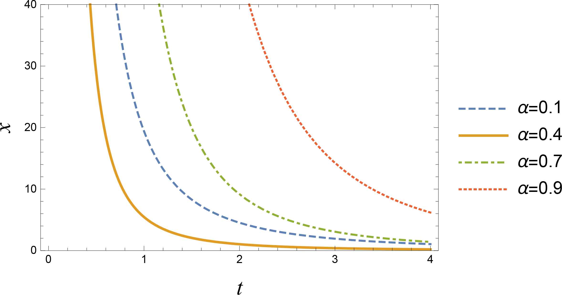
Graphical representation of solutions of fractional Thomas-Fermi equation (3.1) for various values of α.
3.2. Bagley-Torvik Equation
Let us consider the Bagley-Torvik equation [3]
3.2.1. Lie point symmetries
Here, we assume that the Bagley-Torvik equation (3.11) is invariant under the one-parameter Lie group of continuous point transformations (2.6). Thus, the obtained invariant equation is of the form
Substituting
The above equation (3.13) is unsolvable for the arbitrary infinitesimals τ(t, x) and ζ(t, x). In order to find the infinitesimals in equation (3.13), we assume
On solving the last three equations with A ≠ 0 and using τ (0) = 0, we obtain
Substituting (3.19) in (3.14), we obtain
Making use of Laplace transformation on both sides of the equation (3.20) and regrouping the terms, we obtain the following equation
Note that when A ≠ 0, B ≠ 0, C ≠ 0 and f (t) ≠ 0, the infinitesimal generator cannot be written as a linear combination of the space coordinate and the time coordinate. For this reason, the invariant and exact solutions of (3.11) cannot be obtained.
3.2.2. One-dimensional optimal system
In this subsection, we construct a one-dimensional optimal system for the symmetry algebra generated by X1, X2, X3, X4 and X5. In order to obtain the optimal system, we follow the algorithm provided by Olver [48] and Ibragimov [28]. The commutator table for the symmetry generators Xi, i = 1, 2,...,5 is given in Table 1.
| [Xi, Xj] | X1 | X2 | X3 | X4 | X5 |
|---|---|---|---|---|---|
| X1 | 0 | −X2 | −X3 | −X4 | −X5 |
| X2 | X2 | 0 | 0 | 0 | 0 |
| X3 | X3 | 0 | 0 | 0 | 0 |
| X4 | X4 | 0 | 0 | 0 | 0 |
| X5 | X5 | 0 | 0 | 0 | 0 |
Commutator table for infinitesimal generators of equation (3.11)
From the table we observe that the symmetry generators of Bagley-Torvik equation (3.11) form a closed Lie algebra ℒ of dimension five. Now we determine optimal system of one-dimensional subalgebras for (3.11). The adjoint representation of the infinitesimal generators is obtained using the following series
Hence we obtain the adjoint representation of form given in Table 2.
| Ad(exp(∊Xi))Xj | X1 | X2 | X3 | X4 | X5 |
|---|---|---|---|---|---|
| X1 | X1 | e∊X2 | e∊X3 | e∊X4 | e∊X5 |
| X2 | X1 − ∊X2 | X2 | X3 | X4 | X5 |
| X3 | X1 − ∊X3 | X2 | X3 | X4 | X5 |
| X4 | X1 − ∊X4 | X2 | X3 | X4 | X5 |
| X5 | X1 − ∊X5 | X2 | X3 | X4 | X5 |
Adjoint representation for infinitesimal generators of equation (3.11)
Theorem 3.1.
The one-dimensional optimal system of Lie algebra ℒ for the Bagley-Torvik equation (3.11) is X1.
Proof. Define the maps
If a1 ≠ 0, then by taking
3.2.3. Special cases
The special cases for Bagley-Torvik equation (3.11) are discussed below.
Case 1: Let B = 0 and f(t) = 0, t > 0. Then the equation (3.11) reads
Proceeding in the above similar manner, the above equation (3.26) is invariant under
The commutator table for the infinitesimal generators Xi, for i = 1, 2,..., 8, is given in Table 3. By taking k = 1, the linear combinations X2 − X3, X2 + X3, X1 + X4, X1 − X4, X7, X8, 2X5 and −2X6 coincide with the operators obtained for one-dimensional harmonic oscillator equation in [67]. Also, as discussed in [67] the combinations X2 − X3, X1 + X4 and X7 form a compact subalgebra. The Lie symmetries of the second order ODEs are discussed in [2,8,27,49,67].
| [Xi, Xj] | X1 | X2 | X3 | X4 | X5 | X6 | X7 | X8 |
|---|---|---|---|---|---|---|---|---|
| X1 | 0 | 0 | X1 | |||||
| X2 | 0 | 0 | X2 | |||||
| X3 | 0 | 0 | −X3 | |||||
| X4 | 0 | 0 | −X4 | |||||
| X5 | 0 | 0 | ||||||
| X6 | 0 | 0 | ||||||
| X7 | 0 | 0 | ||||||
| X8 | −X1 | −X2 | X3 | X4 | 0 | 0 | 0 | 0 |
Commutator table for infinitesimal generators of equation (3.27)
Construction of exact solution
Consider the infinitesimal generator X = X7 + X1 + X2. Let us assume that F(x, t) is an invariant of equation (3.27), that is
On solving the above equation, we obtain the invariant function
Hence this yields an invariant solution as
Substituting the above invariant solution (3.29) in equation (3.27), we have c1 = 0. Hence, we obtain an exact solution of equation (3.27) as
Case 2: For C = 0 and f(t) = 0, t > 0, the equation (3.11) takes the form
The above equation (3.31) is invariant under
The Lie brackets for the above case are [X1, Xj] = −Xj for j = 2, 3, 4, 5, [Xi, Xj] = 0 for i, j = 2, 3, 4, 5..., and [X1, X1] = 0. In this case the commutator table and adjoint representation are same as that of Tables 1 and 2 respectively.
Note 7. Since the adjoint representation of the infinitesimal operators are same as that of Bagley-Torvik equation (3.11), the one-dimensional optimal system of Lie algebra is X1.
Case 3: Let C = 0,
The commutator table and the adjoint representation of the equation (3.32) take the form same as that of Tables 1 and 2 respectively and hence the one-dimensional optimal system of Lie algebra is X1.
Note 8. We would like to point out that in the above case 2 and case 3, the infinitesimal generator cannot be written as a linear combination of the space coordinate and the time coordinate. For this reason, the invariant and exact solutions of (3.31) and (3.32) cannot be obtained.
3.3. Two-Coupled System of Fractional Quartic Oscillator
Consider the two-coupled system of fractional quartic oscillator as follows
Note that, when α = 1, k3 = 1, k4 = 8 and k5 = 6, the above system (3.33) is known as classical quartic oscillator. The integrability of the classical system was discussed in [35]. It is noteworthy to mention that when α = 1, k3 = −B, k4 = −1, k5 = −A, the above system (3.33) becomes the equations of motion for quartic potential and its detailed discussion can be found in [33].
3.3.1. Lie point symmetries
If the system given by equation (3.33) is invariant under one-parameter Lie group of transformation as given in (2.27), then the invariant equations are as follows
The above invariant system (3.34)–(3.35) is not solvable for arbitrary infinitesimals τ(t, x) and ζ(t, x). Thus, we assume the infinitesimals of the form
Substituting the expression for the infinitesimal
We recall that
Using equations (3.38) and (3.39) in equation (3.37), we obtain
Making use of fractional quartic oscillator equation (3.33) in the above equation (3.40), we obtain
In a similar manner, equation (3.35) can be reduced to
Equations (3.41) and (3.42) reduces to the following overdetermined system of equations
Equation (3.43) subjected to the condition τ(0) = 0 gives
Similarly, from equation (3.44) we obtain
Thus, the two-coupled system of fractional quartic oscillator (3.33) is invariant under
3.3.2. Construction of exact solution
Let F(t, x) be an invariant of equation (3.33). Then
The characteristic equation of the above equation becomes
First we consider
Hence, we obtain the exact solution of the coupled system of fractional quartic oscillator equations (3.33) as
For
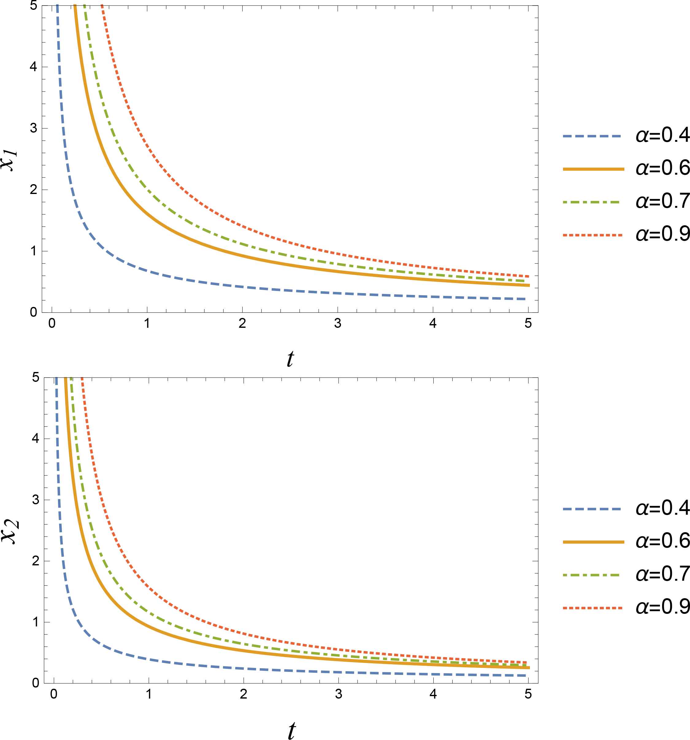
Graphical representations of solutions of fractional system of two-coupled quartic oscillator equation (3.33) for various values of α.
3.4. Fractional Type Coupled Equation of Motion
Consider the following fractional type coupled equation of motion having the form
3.4.1. Lie point symmetries
Assume that the fractional type coupled equation of motion (3.54) is invariant under one-parameter Lie group of transformation (2.27). Then, we obtain the invariant system as
The above system (3.55) is not solvable for τ and
Solving the above system (3.56) with τ(0) = 0, we obtain the infinitesimals as
Thus, the fractional type coupled equation of motion (3.54) is invariant under one-parameter Lie group of transformations
3.4.2. Construction of exact solution
The invariant function F(x, t) of (3.54) reads
Thus, we obtain an exact solution of the fractional type coupled equation of motion (3.54) as follows
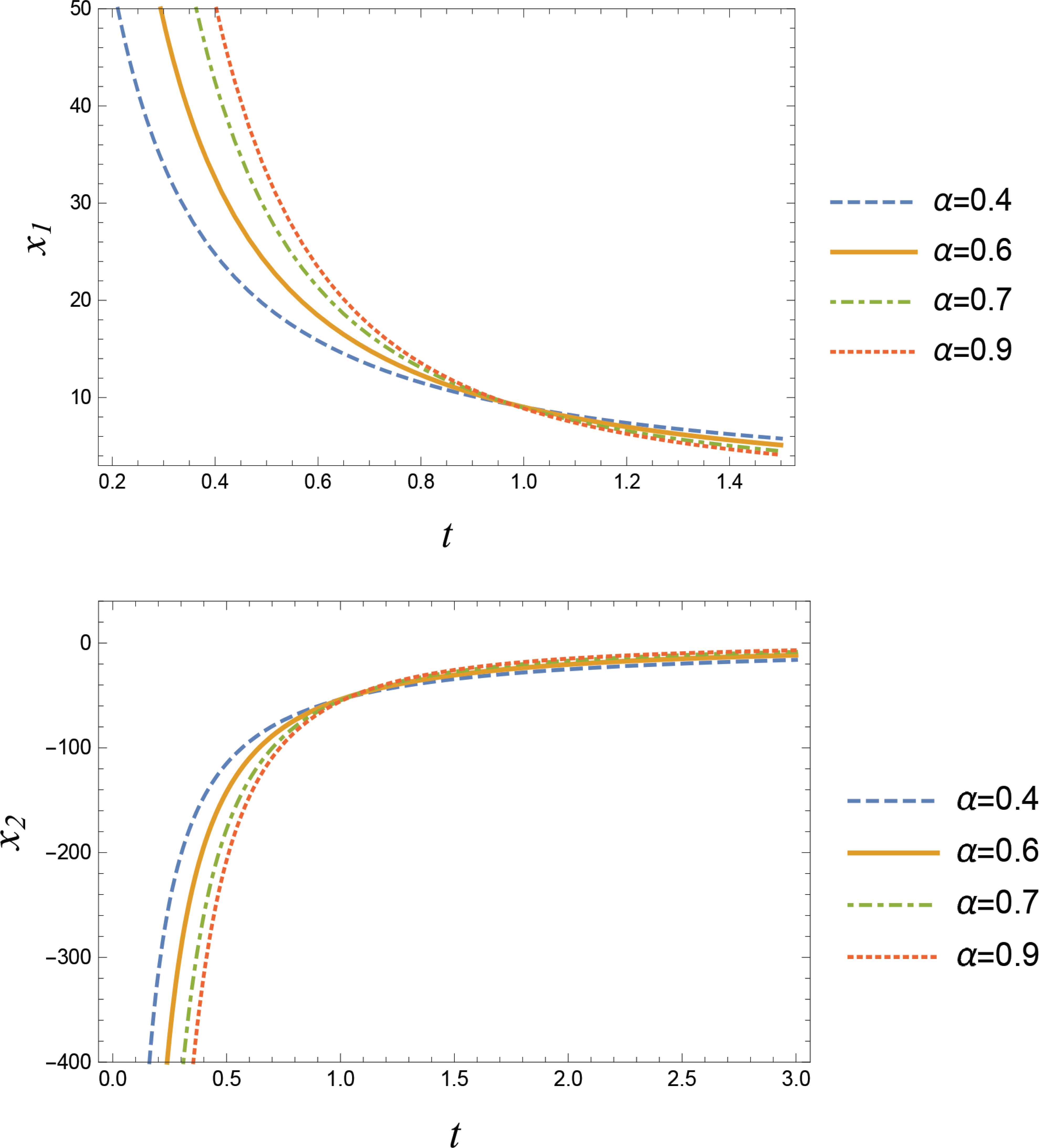
Graphical representations of solutions of fractional type coupled equation of motion for various values of α.
3.5. Fractional Lotka-Volterra ABC System
Consider the following fractional form of Lotka-Volterra ABC system [65]
3.5.1. Lie point symmetries
Assuming that the system (3.58) is invariant under Lie group transformations given in equation (2.27), we get
Let us assume that the infinitesimals
Proceeding in the above similar manner, we obtain
Hence, the fractional Lotka-Volterra ABC system (3.58) is invariant under
Hence, the infinitesimal generator is
3.5.2. Construction of exact solution
The invariant function F of system (3.58) satisfies the equation XF = 0. Hence its characteristic equation becomes
On solving the above characteristic equation, we obtain an exact solution of fractional Lotka-Volterra ABC system (3.58) as
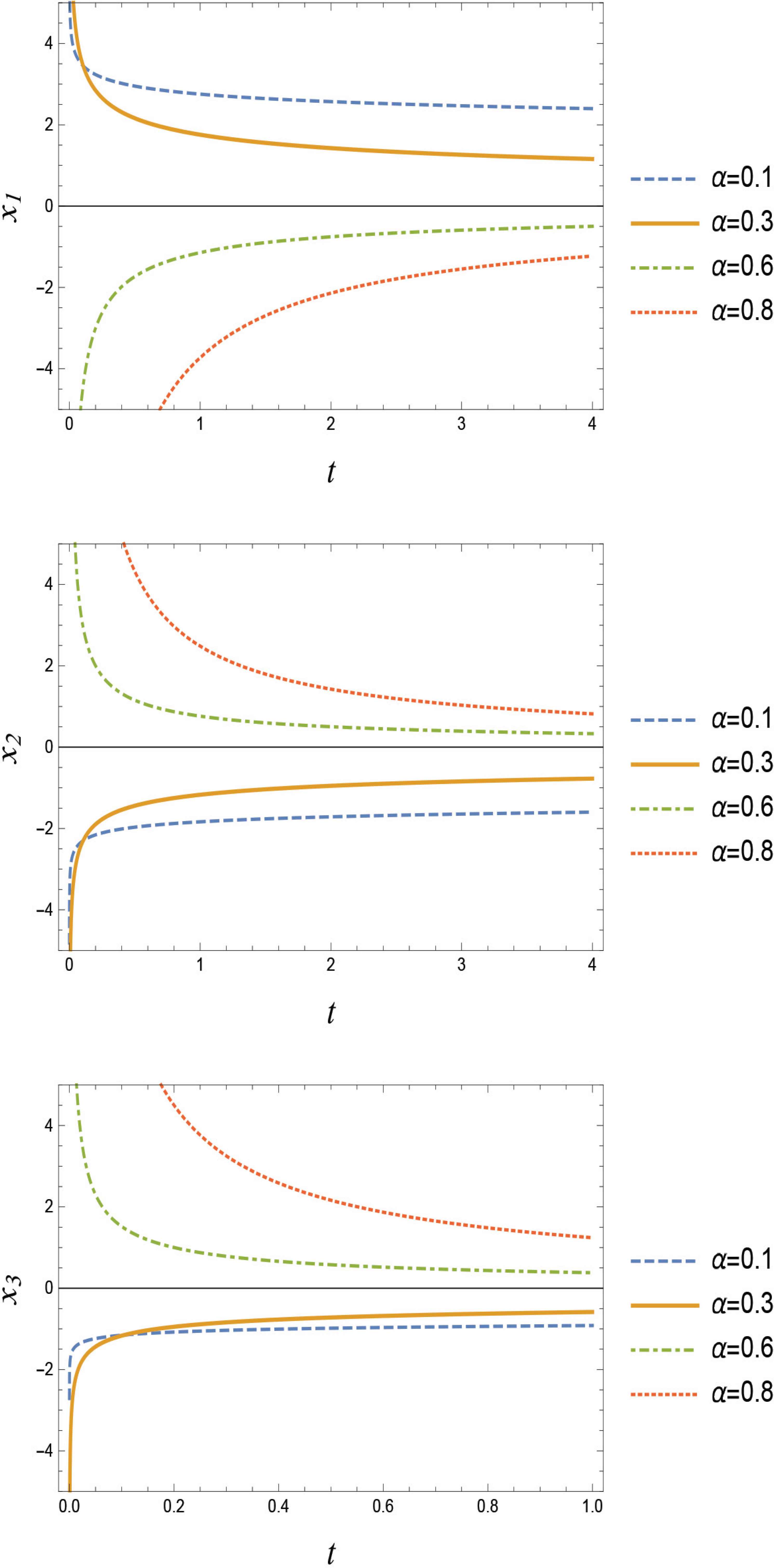
Graphical representation of solutions of fractional Lotka-Volterra ABC system (3.58) for various values of α.
Note 9. Observe that the obtained invariant solutions of the form x(t) ∝ t−α holds only for the R-L fractional derivative because
These type of solutions are not available in the sense of Caputo fractional derivative [32,52].
4. CONCLUDING REMARKS AND DISCUSSION
In this article, we have shown how we can extend the Lie symmetry analysis method for n-coupled system of FODEs with R-L fractional derivative. Also, we systematically presented how to derive the Lie point symmetries of scalar and coupled FODEs namely (i) fractional Thomas-Fermi equation (3.1), (ii) Bagley-Torvik equation (3.12), (iii) two-coupled system of fractional quartic oscillator (3.33), (iv) fractional type coupled equation of motion (3.54) and (v) fractional Lotka-Volterra ABC system (3.58). Furthermore, we explicitly derived the exact solutions of the above mentioned FODEs wherever possible using the obtained Lie point symmetries. The numerical solutions of fractional Thomas-Fermi equation with Caputo derivative was discussed in [12]. In the presented work, we derived the invariant solution of Thomas-Fermi equation (3.1) in the sense of R-L fractional derivative of the form x(t) ∝ t−(α+2). Since the dimensions of the symmetry algebras for Bagley-Torvik equation and its various cases are greater than 2, we constructed the optimal system of one-dimensional subalgebras. We know that the maximal dimension of symmetry algebra for second-order classical ODE is eight. For the second-order Bagley-Torvik equation (3.11), the dimension of symmetry algebra is five due to the presence of R-L fractional derivative of order
We not only extended the Lie symmetry analysis method for n-coupled system of FODEs with R-L fractional derivative but also established the efficiency of the method by solving the two-coupled system of fractional quartic oscillator (3.33), fractional type coupled equation of motion (3.54) and fractional Lotka-Volterra ABC system (3.58). For the system (3.33) the invariant solution
CONFLICTS OF INTEREST
The authors declare they have no conflicts of interest.
ACKNOWLEDGMENT
The authors wish to thank the editors and all the anonymous reviewers for their fruitful comments and suggestions for the significant improvement of the manuscript.
REFERENCES
Cite this article
TY  - JOUR
AU  - K. Sethukumarasamy
AU  - P. Vijayaraju
AU  - P. Prakash
PY  - 2021
DA  - 2021/03/31
TI  - On Lie Symmetry Analysis of Certain Coupled Fractional Ordinary Differential Equations
JO  - Journal of Nonlinear Mathematical Physics
SP  - 219
EP  - 241
VL  - 28
IS  - 2
SN  - 1776-0852
UR  - https://doi.org/10.2991/jnmp.k.210315.001
DO  - 10.2991/jnmp.k.210315.001
ID  - Sethukumarasamy2021
ER  -