Journal of Nonlinear Mathematical Physics

Volume 25, Issue 4, July 2018, Pages 528 - 557

Composition of Lie Group Elements from Basis Lie Algebra Elements

Authors
George W. Bluman
Department of Mathematics, University of British Columbia, Vancouver V6T 1Z2, Canada,bluman@math.ubc.ca
Omar Mrani-Zentar
Department of Mathematics, University of British Columbia, Vancouver V6T 1Z2, Canada,o.mrani@math.ubc.ca
Deshin Finlay
Department of Mathematics, University of Michigan, Ann Arbor 48109-1043, USA,dfinlay@umich.edu
Received 15 June 2017, Accepted 27 April 2018, Available Online 6 January 2021.
DOI
10.1080/14029251.2018.1503398How to use a DOI?
Keywords
Lie groups; Lie algebras; commutators
Abstract

It is shown explicitly how one can obtain elements of Lie groups as compositions of products of other elements based on the commutator properties of associated Lie algebras. Problems of this kind can arise naturally in control theory. Suppose an apparatus has mechanisms for moving in a limited number of ways with other movements generated by compositions of allowed motions. Two concrete examples are: (1) the restricted parallel parking problem where the commutator of translations in y and rotations in the xy-plane yields translations in x. Here the control problem involves a vehicle that can only perform a series of translations in y and rotations with the aim of efficiently obtaining a pure translation in x; (2) involves an apparatus that can only perform rotations about two axes with the aim of performing rotations about a third axis. Both examples involve three-dimensional Lie algebras. In particular, the composition problem is solved for the nine three- and four-dimensional Lie algebras with non-trivial solutions. Three different solution methods are presented. Two of these methods depend on operator and matrix representations of a Lie algebra. The other method is a differential equation method that depends solely on the commutator properties of a Lie algebra. Remarkably, for these distinguished Lie algebras the solutions involve arbitrary functions and can be expressed in terms of elementary functions.

Copyright
© 2018 The Authors. Published by Atlantis and Taylor & Francis
Open Access
This is an open access article distributed under the CC BY-NC 4.0 license (http://creativecommons.org/licenses/by-nc/4.0/).

1. Introduction

Lie groups and their representations play an important role in various applications. Lie groups of transformations describe rigid body motions (rotations and translations), scalings, as well as other transformations. In this paper it is shown explicitly how one can obtain basis elements of Lie groups as compositions of products of other basis elements, motivated by the commutator properties of associated Lie algebras. Problems of this kind can arise naturally in control theory [3, 8, 9]. Here an apparatus has mechanisms for moving in a limited number of ways and the aim is to generate efficiently other movements from compositions of possible motions. Two concrete examples are: (1) the restricted parallel parking problem where the commutator of translations in y and rotations in the xy-plane yields translations in x. Here the control problem involves a vehicle that can only perform translations in y and rotations with the aim of efficiently obtaining a pure translation in x;(2) involves an apparatus that can only perform rotations about two axes with the aim of generating rotations about a third axis. Here the commutator of rotations about two axes yields rotations about the third axis. Both examples involve three-dimensional Lie algebras. In terms of the notation used in [11], examples (1) and (2) respectively include the Lie algebras S3,3 with its parameter set to zero and so (3,). The authors are unaware of literature that has solved this composition problem.

Three distinct methods are presented to solve the composition problem. The first method (operator method) depends on realizing a Lie group as a Lie group of transformations. Such realizations can be found in [6] for some and in [10] for all three- and four-dimensional Lie algebras.

The second method (matrix representation method) involves matrix representations of finite-dimensional Lie algebras which are known to exist from Ado’s theorem [1]. This theorem states that there exists a faithful square matrix representation for every finite-dimensional Lie algebra. There are many existing algorithms that generate such matrices including one developed by Willem de Graaf [7] . While the minimal dimension of a matrix representation is not known in general, it is known for three- and four-dimensional Lie algebras (see [4] and [5]). This method is also applied to a control theory problem in [8]

The third method (DE method) was initially presented in [2] for other purposes. This method only uses the commutator properties of a Lie algebra. In particular, it does not require the use of a representation of a Lie algebra. The DE method involves setting up and solving an initial value problem for a nonlinear system of first order ordinary differential equations. The DE method yields a necessary condition for solutions—it turns out that for all three- and four-dimensional cases, the DE method yields all solutions.

Remarkably, for all relevant n -dimensional Lie algebras, n = 3 or 4, when the considered composition has n + 1 Lie group elements, the solution involves one arbitrary function and can be expressed in terms of elementary functions.

In Section 2, we give a precise mathematical statement of the research problem. Then we describe fully the three different methods used to solve it. As an illustrative example, we focus on the Lie algebra sl(2, F). In Section 3, in two tables we summarize our results for all relevant three- and four-dimensional Lie algebras. Following this, we show the essential details that yield these solutions. Finally in Section 4, we make further remarks and discuss the advantages and disadvantages of the three presented methods.

2. Research problem

Consider a three-dimensional Lie algebra L, if B1, B2, and B3 form a basis for L then the commutator of B1 and B2 is a linear combination of the basis elements of L, i.e.,

[B1,B2]=B1B2B2B1=k=13C12kBk,(2.1)
in terms of real structure constants C121, C122 and C123. For the research problem under consideration we require that C1230. In other words, the Lie algebra element B3 is generated by the other two elements. All six three-dimensional Lie algebras presented in [11] have at least one commutator that satisfies this property. In particular, for the problem under consideration, it does not matter what the other commutators of L are. The question of interest is whether the Lie group element generated by B3 can be obtained from the Lie group elements generated by B1 and B2 as illustrated by the two examples mentioned in the introduction. Motivated by the commutator property (2.1) with C1230, the aim is to find continuous functions a(ε), b(ε), c(ε) and d(ε) so that the equation
ea(ε)B1eb(ε)B2ec(ε)ced(ε)B2=eεB3
with
a(0)=b(0)=c(0)=d(0)=0(2.2)
holds for an arbitrary value of ε. Next, to clarify how the research problem given by (2.2) follows from (2.1) with C1230 a concrete example is presented.

The parallel parking problem has commutators given by [R, Y] = X, [R, X] = − Y, [X, Y] = 0, where

X=x,Y=y,R=yxxy.
The first commutator indicates that X can be generated from R and Y. This leads one to consider either equation
ea(ε)Reb(ε)Yec(ε)Red(ε)Y=eεX;(2.3)
or
ea(ε)Yeb(ε)Rec(ε)Yed(ε)R=eεX.(2.4)
In this example R, Y, and X correspond to B1, B2, and B3 respectively. The solution to equation (2.3) will be presented in Section 3. Note that when the commutator of the Lie algebras used in equation (2.2) do not satisfy the assumptions stated above, one would not expect any non-trivial solutions. For example, since in the parking problem the commutators of X and Y do not generate R, the equation
ea(ε)Xeb(ε)Yec(ε)Xed(ε)Y=eεR
does not have a non-trivial solution.

When the DE method is used, additional assumptions about these functions are needed. In particular, here a(ε), b(ε), c(ε) and d(ε) are differentiable everywhere except at ε = 0. This assumption is needed since the DE method relies on finding a system of differential equations that the four functions must satisfy.

In general, it turns out that the problem as stated will always have a degree of freedom in its solution. Moreover, a minimum number of four terms are needed on the left hand side of equation (2.2). This follows from the origin of the commutator equation (2.1). In particular, from the form of equation (2.2), one would expect, as will be seen later in this paper, that there are solutions for which a(ε), b(ε), c(ε) and d(ε) are of order ε as ε → 0 in order to generate a commutator element of order ε on the right-hand side of equation (2.2)

Now consider a four-dimensional Lie algebra L with basis elements B1, B2, B3, and B4 such that the elements B1, B2, and B3 do not form a subalgebra. For the research problem we require that the commutator of B1 and B2 satisfies

[B1,B2]=B1B2B2B1=k=14C12kBk,(2.5)
with real structure constants C121,,C124 where C1230 and C124=0. Here the Lie algebra element B3 can be generated from the elements B1 and B2. The problem of interest is whether the Lie group element generated by B3 can be obtained from the Lie group elements generated by B1 and B2. In particular, in view of the commutator property (2.5), we are interested in finding continuous functions a(ε), b(ε), c(ε) and d(ε), f(ε), and g(ε) so that the equation
ea(ε)B1eb(ε)B2ec(ε)B1ed(ε)B2ef(ε)B1eg(ε)B2=eεB3,(2.6)
with a(0) = b(0) = c(0) = d(0) = f(0)) = g(0) = 0 holds for an arbitrary value of ε.

It is essential to note that the left hand side of (2.6) is composed of the product of six Lie group elements: in all considered cases there exist solutions where one of a(ε) or g(ε) is zero, but this is not determinate a priori.

One should also note that one can state the problems in (2.2) and (2.6) with the roles of B1 and B2 interchanged when the number of terms to the left of these equations is even. This does not change the nature of the problem. For the Lie algebras where both problems were considered, it was found that they led to isomorphic solutions.

In this paper, for all relevant three- and four-dimensional Lie algebras, we present three different methods that can yield the general solution for their respective equations (2.2) and (2.6). In what follows, we will describe the different methods used to solve (2.2) and (2.6). As a simple example, in this section we solve the composition problem for the three-dimensional Lie algebra sl(2, F) to illustrate how these different methods work. The solution of the composition problem for the other relevant three- and four-dimensional Lie algebras will be presented in Section 3.

We first note that sl(2, F) has the commutators

[X,Y]=Z,[Z,X]=2X,[Y,Z]=2Y.(2.7)

2.1. Operator method

The operator method requires a representation of a Lie algebra in terms of differential operators. The operator representation is not necessarily unique. This lack of uniqueness is illustrated by the example of sl(2, F).

2.1.1. Description of the procedure for the operator method

Let {Δ1,…,Δk} be a differential operator representation of a Lie algebra L which respectively has basis elements {B1,…,Bk}, where

Δi=γji(x)xj,i=1,,k, and x=(x1,,xm).

Then equations (2.2) and (2.6) become respectively the equations

ea(ε)Δ1eb(ε)Δ2ec(ε)Δ1ed(ε)Δ2x=eεΔ3x,(2.8)
and
ea(ε)Δ1eb(ε)Δ2ec(ε)Δ1ed(ε)Δ2ef(ε)Δ1eg(ε)Δ2x=eεΔ3x(2.9)
where eεΔix=n=0εnn!Δinx=(xi) for i = 1, . . . , k; (xi)=((x1i),,(xmi)) is the image of x with respect to the ith basis element of the Lie group of transformations connected with the differential operator Δi, i = 1,…,k.

From the First Fundamental Theorem of Lie, one can also obtain (xi)* by solving the system of differential equations

d(xji)dε=γji(x),j=1,,m, with initial condition (xji))(0)=xj.

2.1.2. Example sl(2, F)

Operator representations for sl(2, F) include

Δ1=X=x2x, Δ2=Y=x, Δ3=Z=2xx, in ;(2.10)
Δ1=X=yx, Δ2=Y=xy, Δ3=Z=yyxx, in 2.(2.11)

For the operator representation (2.10) for sl(2, F), one obtains

eεX(x)=x1+εx,eεY(x)=x+ε,eεZ(x)=e2εx.(2.12)

There are two well-known methods to obtain (2.12).

Method I. From the First Fundamental Theorem of Lie, the operator representation (2.10) leads to solving separately the three IVPs

dxdε=x2,x(0)=x;(2.13)
dxdε=1,x(0)=x;(2.14)
dxdε=2x,x(0)=x.(2.15)
It is easy to show that the three Lie group transformations (2.12) respectively solve the IVPs (2.13)(2.15).

Method II. Using induction, it is easy to show that Xnx=(1)nn!xn+1,n0. Hence eεXx=n=0enn!Xnx=n=0εn(1)nxn+1=x1+ex. Since Y x=1, Yn x = 0, n ≥ 2, it follows that eεY x = x + ε. It is easy to show that Znx = 2nx, n ≥ 0. Hence eεZx = e2εx.

To proceed, it is convenient to rewrite expression (2.8) in the form

eb(ε)Yec(ε)Xed(ε)Yx=ea(ε)XeεZx.(2.16)
Then from (2.12), one obtains
eb(ε)Yec(ε)Xed(ε)Yx=eb(ε)Yec(ε)X(x+d)=eb(ε)Y(d+x1+cx)=d+x+b1+c(x+b),ea(ε)XeεZ(x)=ea(ε)X(e2εx)=e2εx1ax.
Then expression (2.16) becomes d+x+b1+c(x+b)=e2εx1ax. Hence for all x, one has
(a(dc+1)+ce2ε)x2+(a(d+b+bdc)+dc+1e2ε(1+bc))x+b+d+bdc=0.
This yields the set of equations
b+d+bdc=0, dc+1=e2ε(1+bc), a(dc+1)=ce2ε.(2.17)
The solution to the system of equations (2.17) is given by
a(ε)=eεe2εd(ε),b(ε)=eεd(ε),c(ε)=eε1d(ε),(2.18)
where d(ε) is any continuous function chosen so that a(ε) and c(ε) are continuous functions, and satisfying d(ε) ≠ 0 for any ε ≠ 0 with a(0) = b(0) = c(0) = d(0) = 0.

2.2. Matrix representation method

The matrix representation method involves a matrix representation of L. In particular, one seeks an appropriate matrix for each basis element of L using the Lie algebra package of the computer software GAP (Group, Algorithms, Programming) [7]. A difficulty arose in the case of the four-dimensional Lie algebra S4,7 (in terms of the nomenclature used in the classification of Lie algebras in [11]). Here the matrix representation obtained from the software package [7] could not be used since the obtained representation is not isomorphic to S4,7. For this Lie algebra, we used a matrix representation given in [4].

2.2.1. Description of the procedure used for the matrix representation method

Let L be a k-dimensional Lie algebra with basis elements Bi with Mi denoting a matrix representation of Bi, i = 1,…,k.

Step 1. Find matrices {Mi} that represent L using computer software or relevant literature ([4],[7]).

Step 2. Attempt to find a closed form representation for each element eεBi of the Lie group associated with L from the Taylor expansion eεMi=n=0εnn!Min where Mi0=I for i =1,…,k. (In all three- and four-dimensional cases, this step was successful in leading to such a closed form representation.)

Step 3. Compute where i=12k2eai(ε)Bj where{j=1 if i is odd, j=2 if i is even.

Step 4. Solve equations (2.2) and (2.6).

2.2.2. Example sl(2, F)

Although sl(2, F) is a three-dimensional Lie algebra, a matrix representation is given by the 2 × 2 matrices X=(0100), Y=(0010), Z=(1001). Then X2=(0000). Hence Xn=(0000), n ≥ 2. Thus eεX=I+εX=(1ε01). Similarly, one can show that eεY=(10ε1). One can easily show that Zn=(100(1)n). Hence eεZ=(eε00eε). Consequently,

M=ea(ϵ)Xeb(ϵ)Yec(ϵ)Xed(ϵ)Y=(abcd+ab+ad+cd+1a+c+abcb+d+bcdbc+1).  
After setting M=eεZ, one obtains the equations
bc+1=eε,b+d+bcd=0,a+c+abc=0,abcd+ab+ad+cd+1=eε,
whose solution is given by (2.18).

2.3. DE method

The DE method requires differentiation of the unknown functions in equations (2.2) and (2.6). It involves setting up a nonlinear system of first order ordinary differential equations that must be satisfied by all differentiable solutions of equations (2.2) and (2.6). Here the solutions respectively satisfy initial conditions

a(0)=b(0)=c(0)=d(0)=0,(2.19)
a(0)=b(0)=c(0)=d(0)=f(0)=g(0)=0(2.20)
in the three- and four-dimensional cases. Note that when ε = 0, the unknown functions will be continuous but not differentiable. The DE method yields a necessary condition for solutions. Sufficiency is shown from the solutions obtained by the other two methods.

2.3.1. Description of the procedure used for the DE method

After differentiating equations (2.2) and (2.6) with respect to ε, one obtains respectively,

a1(ε)B1i=14eaiBi+a2(ε)ea1B1B2i=24eaiBi+a3(ε)i=12eaiBiB1i=34eaiBi+a4(ε)i=13eaiBiB2ea4B2=B3eεB3,(2.21)
a1(ε)B1i=16eaiBi+a2(ε)ea1B1B2i=26eaiBi++a6(ε)i=15eaiBiB2ea6B2=B3eεB3,(2.22)
where Bi={B1 if i is odd B2 if i is even  and a1 = a, a2 = b, a3 = c, a4 = d, a5 = f, a6 = g.

From equations (2.21) and (2.22), one sees that a formula is needed for pulling the products of the exponentials appropriately to the right of each Bp in order to get back i=1neai(ε)Bi=eεB3, n = 4, 6, respectively.

In general, one proceeds as follows.

Step 1. Find {fj}so that

eεBiBp=j=1kfjBjeεBi(2.23)
where i = 1, 2, p = 1, · · · , k, and k is the dimension of the Lie algebra L. Since Ado’s theorem [7] guarantees the existence of a matrix representation for every finite-dimensional Lie algebra, one can treat the operations in L as matrix elements so that, without loss of generality, L is associative.

Step 2. Differentiate equations (2.2) and (2.6) with respect to ε to obtain equations (2.21) and (2.22), respectively. Then appropriately and recursively substitute equation (2.23) into equations (2.21) and (2.22). Thus in each case one obtains an equation of the form

j=1kαj(ε)Bji=1keaiBi=B3eεB3,(2.24)
for specific functions αj(ε).

Step 3. Assume that expressions (2.2) and (2.6) hold. Consequently, this yields necessary conditions that {αj(ε)} must satisfy, namely the nonlinear system of first order ODEs

α3(ε)=1αi(ε)=0,i3,(2.25)
with initial conditions (2.19) and (2.20), respectively.

Step 4. Check that the solution of the ODE system (2.25) solves respectively expressions (2.2) or (2.6) using either the matrix or operator method.

2.3.2. Example sl(2,F)

Theorem 2.1.

For sl(2,F) these identities hold for any ε.

eεXY(Y+εZε2X)eεX, eεXZ(Z2εX)eεX, eεYX(XεZε2Y)eεY,eεYZ=(Z+2εY)eεY.(2.26)

Proof. From the commutator relations (2.7), one directly obtains

XY=YX+Z,XZ=ZX2X,YZ=ZY+2Y.
Hence X2Y = YX2 + 2 ZX−2X. Then it is easy to show that
XnY=YXn+nZXn1n(n1)Xn1,n.
Similarly, one can show that the following relations hold.
XnZ=ZXn2nXn,YnX=XYnnZYn1n(n1)Yn1,YnZ=ZYn+2nYn.
Consequently,
eεXY=YeεX+εZn=1εn1(n1)!Xn1ε2Xn=2εn2(n2)!Xn2=(Y+εZε2X)eεX.
Similarly, one obtains the remaining relations in (2.26), completing the proof.

Now to proceed further, we differentiate equation (2.6) with respect to ε. This yields

a(ε)XeεZ+b(ε)ea(ε)XYeb(ε)Yed(ε)Y+c(ε)ea(ε)Xeb(ε)YXec(ε)Xed(ε)Y+d(ε)ea(ε)Xeb(ε)Yec(ε)XYed(ε)Y=Ze(ε)Z.(2.27)
Using the relations in Theorem 2.1 , one finds that equation (2.27) becomes [α1(ε)X + α2(ε)Y + α3(ε) Z] eεZ = Z eεZ with
α1(ε)=aa2(b+d+b(bc+bc2d+2cd))+c+2abc2acdc2d2abc2d=0,(2.28)
α2(ε)=b+d+b(bc+bc2d+2cd)=0,(2.29)
α3(ε)=a(b+d+b(bc+bc2d+2cd))bc+cd+bc2d=1.(2.30)
After substituting equation (2.29) into equations (2.28) and (2.30), one gets respectively
a+cc2d2a(bc+cd+bc2d)=0,(2.31)
bc+cd+bc2d=1.(2.32)
After substituting equation (2.32) into each of equations (2.31) and (2.29), one obtains
a+cc2d2a=0,(2.33)
b+d+bcd+b=0.(2.34)
After subtracting c times equation (2.34) from equation (2.32), one finds that (bc)′+ bc = − 1 Hence
b(ε)=eε1c(ε).(2.35)
Substitution of equation (2.35) into equation (2.34) leads to d=ceεc(e1)c2.

Consequently,

d(ε)=eε1c(ε).(2.36)
After substituting equation (2.36) into equation (2.33), one gets

2(a + eεc) = (a + eεc)′. Hence a(ε) = − c(ε)eε .

Thus the solution to the system of differential equations (2.25)(2.27) with initial condition (2.16) is given by (2.18).

3. Results

Using the procedures described in Section 2, the results for all relevant three- and four-dimensional Lie algebras are presented in Tables 1 and 2, respectively.

Lie algebra; commutators Composition equation Solution
sl(2, F)
[X, Y] = Z
[X, Z] = −2X
[Y, Z] = 2Y
ea(ε)Xeb(ε)Yec(ε)Xed(ε)Y=eεZ d(ε) is an arbitrary function satisfying d(ε) ≠ 0 when ε ≠ 0
a(ε)=eεe2εd(ε)b(ε)=eε1eε1d(ε)c(ε)=eε1d(ε)
Parallel parking problem, S3,3 with constant r = 0
[R, Y] = X
[R, X] = −Y
[X, Y] = 0
ea(ε)Reb(ε)Yec(ε)Red(ε)Y=eεX c(ε) is an arbitrary function satisfying c(ε) ≠ for every k ∈ ℤ when ε ≠ 0
a(ε) = −c(ε)
b(ε) = −εcsc c(ε)
d(ε) = ε cot c(ε)
Euler angles problem, so(3,ℝ)
[X, Y] = Z
[X, Z] = −Y
[Y, Z] = X
ea(ε)Xeb(ε)Yec(ε)Xed(ε)Y=eεZ Any c(ε) satisfying c(ε) ≠ for every k ∈ ℤ when ε ≠ 0 and |sinεsinc(ε)|1 with a(ε)=arccos(cosc(ε)cosε)b(ε)=arcsin(sinεsinc(ε))d(ε)=arccos(sina(ε)sinc(ε));a(ε)=arccos(cosc(ε)cosε)b(ε)=π+arcsin(sinεsinc(ε))d(ε)=arccos(sina(ε)sinc(ε))
n3,1
[X, Y] = Z
[X, Z] = 0
[Z, Y] = 0
ea(ε)Xeb(ε)Yec(ε)Xed(ε)Y=eεZ d(ε) is an arbitrary function satisfying d(ε) ≠ 0 when ε ≠ 0
a(ε)=εd(ε)b(ε)=d(ε)c(ε)=εd(ε)
S3,1
[Y, Z] = −Y
[Y, X] = 0
[Z, X] = rX + Y
where r is a constant satisfying |r| ≤ 1
ea(ε)Xeb(ε)Zec(ε)Xed(ε)Z=eεY d(ε) is an arbitrary function satisfying d(ε) ≠ 0 when ε ≠ 0
b(ε)=d(ε)a(ε)=ε(1r)1e(r1)d(ε)c(ε)=a(ε)erd(ε)
S3,2
[Z, X] = X
[Z, Y] = X +Y
[X, Y] = 0
ea(ε)Yeb(ε)Zec(ε)Yed(ε)Z=eεX d(ε) is an arbitrary function satisfying d(ε) ≠ 0 when ε ≠ 0
b(ε)=d(ε)a(ε)=εed(ε)d(ε)c(ε)=εd(ε)
S3,3 general case
[R, X] = rXY
[R, Y] = X + rY
[X, Y] = 0
where r is a non-negative constant.
ea(ε)Reb(ε)Yec(ε)Red(ε)Y=eεX c(ε) is an arbitrary function satisfying c(ε) ≠ for every k ∈ ℤ when ε ≠ 0
a(ε) = −c(ε)
b(ε) = − εcsc c(ε)erc(ε)
d(ε) = ε cot c(ε)
Table 1:

Results for three-dimensional Lie algebras

Lie algebra; commutators Composition equation Solution
S4,2
[W, X] = X
[W, Y] = X + Y
[W, Z] = Y + Z
[X, Y] = 0
[X, Z] = 0
[Z, Y] = 0
ea(ε)Web(ε)Zec(ε)Wed(ε)Zef(ε)W=eεY c(ε) is an arbitrary function satisfying c(ε) ≠ 0 when ε ≠ 0
a(ε)=f(ε)=12c(ε)b(ε)=εc(ε)e12c(ε)d(ε)=εc(ε)e12c(ε)
S4,7
[Y, Z] = X
[W, Y] = −Z
[W, Z] = Y
[W, X] = 0
[X, Y] = 0
[X, Z] = 0
ea(ε)Zeb(ε)Wec(ε)Zed(ε)Wef(ε)Z=eεY b(ε) is an arbitrary function satisfying b(ε) ≠ for every k ∈ ℤ when ε ≠ 0
a(ε)=ε2tanb(ε)c(ε)=εsinb(ε)d(ε)=b(ε)f(ε)=ε2tanb(ε)
S4,9
[Y, Z] = X
[W, Y] = rYZ
[W, Z] = Y + rZ
[W, X] = 2rX
[X, Y] = 0
[X, Z] = 0
ea(ε)Web(ε)Zec(ε)Wed(ε)Zef(ε)W=eεY b(ε) is an arbitrary function satisfying b(ε) ≠ for every k ∈ ℤ

when ε ≠ 0
a(ε)=ε2tanb(ε)c(ε)=εerbsinb(ε)d(ε)=b(ε)f(ε)=ε2tanb(ε)
S4,10
[Y, Z] = X
[W, Y] = Y
[W, Z] = Y + Z
[W, X] = 2X
[X, Y] = 0
[X, Z] = 0
ea(ε)Web(ε)Zec(ε)Wed(ε)Zef(ε)Weg(ε)Z=eεY a(ε) and c(ε) are arbitrary functions satisfying a(ε)c(ε) ≠ 0, a(ε) + c(ε) ≠ 0, and c(ε)2 + a(ε)c(ε) ≥ 0
f(ε)=(a(ε)+c(ε))b(ε)=ε(c(ε)±c(ε)2+a(ε)c(ε)a(ε)c(ε))ea(ε)g(ε)=ε+b(ε)c(ε)ea(ε)a(ε)+c(ε)d(ε)=g(ε)e(a(ε)+c(ε))b(ε)ec(ε)
and in the limiting case when
a(ε)=0,f(ε)=c(ε)d(ε)=εec(ε)c(ε)b(ε)=g(ε)=ε2c(ε)
Table 2:

Results for four-dimensional Lie algebras

The sketch of the proofs of the results, exhibited in Tables 1 and 2, follow.

3.1. Parallel parking problem (Lie algebra S3,3 with constant r = 0)

3.1.1. Model example

To illustrate parallel parking, as an example, consider a unicycle that performs forward and backward translations as well as rotations. The unicycle is represented by a straight line with centre located at (x,y) and initial orientation parallel to the y-axis with its centre located at (0,0) in Figure 1. The aim is to move the unicycle so that its centre finishes at (ε, 0) with the vehicle parallel to its initial orientation by a succession of rotations and translations in the same direction as the straight line. As will be illustrated in Figure 1, the minimum number of steps that start with a nonzero translation is four. Let d(ε) and b(ε) be the translations in the first and third steps, respectively and let c(ε) and a(ε) be the angles of rotation in the second and last steps, respectively. Since the direction the vehicle is facing at the end must be the same as at the start, one must have a(ε) = −c(ε). From Figure 1, one sees that d(ε) + b(ε) cos c(ε) = 0 and b(ε) sin c(ε) = ε . Hence the solution to this problem is given by

a(ε)=c(ε), b(ε)=εsinc(ε), d(ε)=εcotc(ε),(3.1)
where c(ε) is any continuous function chosen so that b(ε) and d(ε) are continuous functions, and satisfying c(ε) ≠ for every k and ε ≠ 0 with a(0) = b(0) = c(0) = d(0) = 0.

Fig. 1:

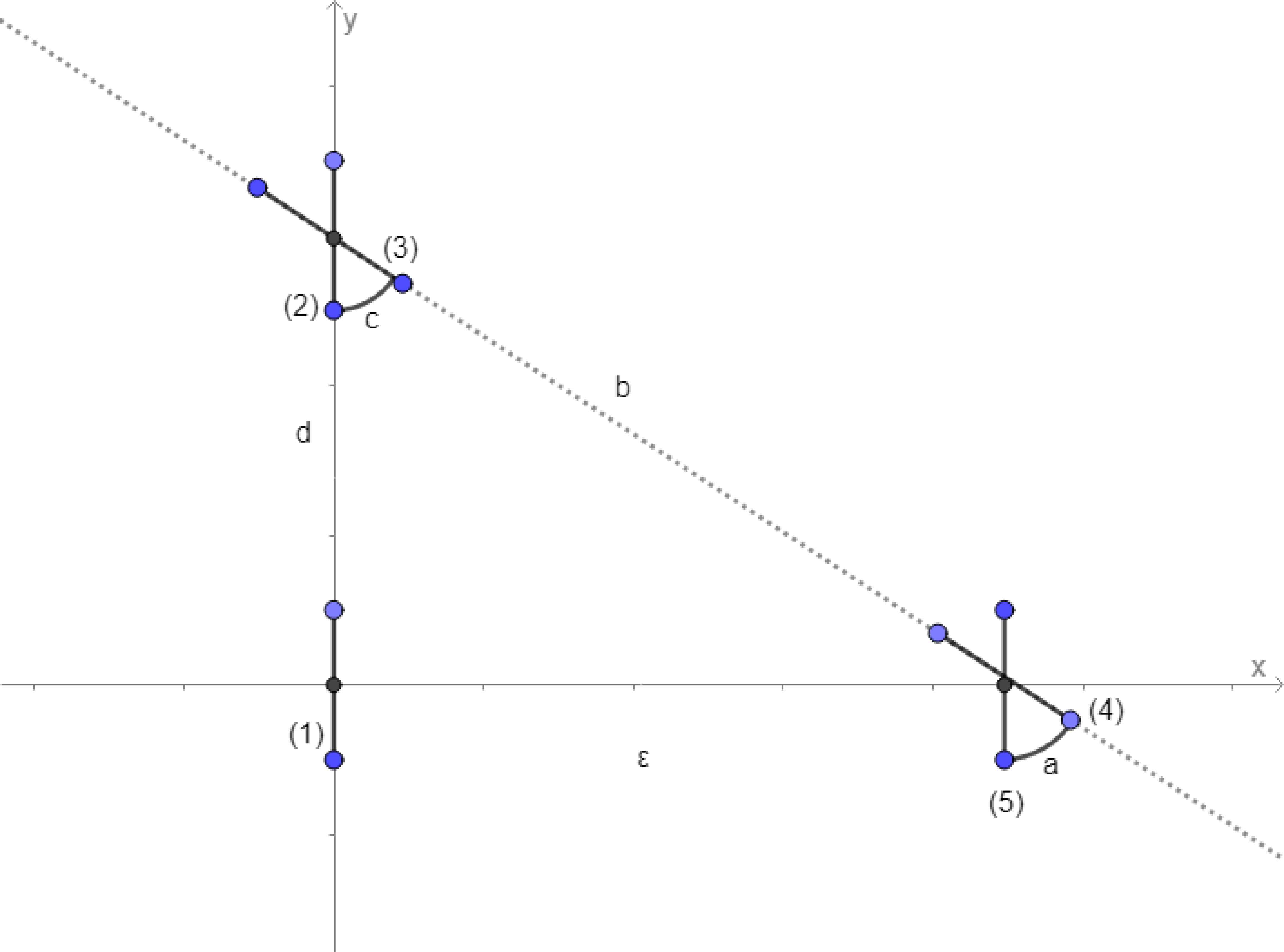
Illustration of solution of parallel parking problem. (1) represents initial configuration of vehicle with successive configurations represented by (2) to (5).

Alternatively, one could treat d(ε) as an arbitrary function. Here the solution as reflected by Figure 1 is given by

a(ε)=c(ε),c(ε)=arctan(εd), |b(ε)|=d2+ε2,
where d(ε) is any continuous function chosen so that c(ε) is a continuous function, and satisfying d(ε)0 and 2πε<d(ε)<2πe for every ε ≠ 0 with a(0) = b(0) = c(0) = d(0) = 0.

Next, the solution to the parallel parking problem is presented using the methods described in Section 2 which can be applied to any Lie algebra.

3.1.2. Solution using the operator method

An operator representation for this Lie algebra is given by

X=x, Y=y, R=yxxy.
Consequently,
M=ea(ε)Reb(ε)Yec(ε)Red(ε)Y(x,y)=ea(ε)Reb(ε)Yec(ε)R(x,y+d)=ea(ε)Reb(ε)Y(xcosc+ysinc,d+ycoscxsinc)=ea(ε)R(bsinc+xcosc+ysinc,d+bcosc+ycoscxsinc)=(bsinc+xcos(a+c)+ysin(a+c),d+bcoscxsin(a+c)+ycos(a+c)).
Then M = eεX(x,y) = (xε,y) iff
sin(a+c)=0, cos(a+c)=1, d+bcosc=0, bsinc=ε.(3.2)

The solution to the system of equations (3.2) is given by (3.1).

3.1.3. Solution using the matrix representation method

A matrix representation of S3,3 with constant r = 0 is given by

X=(001000000),Y=(000001000),R=(010100000).
Hence Xn = Yn = 0, n ≥ 2.

Thus eεY=I+εY=(10001ε001), and eεX=(10ε010001).

For all k > 0, one has

(010100000)k={(010100000)if k=1(mod4)(100010000)if k=2(mod4)(010100000)if k=3(mod4)(100010000)if k=4(mod4)
Consequently,
eεR=(cosεsinε0sinεcosε0001).
Hence
M=ea(ε)Reb(ε)Yec(ε)Red(ε)Y=(cos(a+c)sin(a+c)dsin(a+c)+bsinasin(a+c)cos(a+c)dcos(a+c)bcosa001).
Then M = eεX is satisfied iff
cos(a+c)=1, sin(a+c)=0, bsina=ε, d+bcosa=0.(3.3)

The solution to the system of equations (3.3) is given by (3.1).

3.1.4. Solution using the DE method

For all n ≥ 0, one can show that

XnY=YXn, XnR=RXnnYXn1,RnX=Xi=0i evenn(1)i2(ni)RniYi=1i odd n(1)i+12(ni)Rni,RnY=Yi=0i evenn(1)i2(ni)Rni+Xi=1i odd n(1)i+12(ni)Rni .(3.4)

Using these results, one can easily obtain the identities

eεYXXeεY,eεYR(RεX)eεY,eεRX(cosεXsinεY)eεR,eεRY(cosεY+sinεX)eεR.(3.5)

Now to proceed, we differentiate with respect to ε the equation

ea(ε)Reb(ε)Yec(ε)Red(ε)Y=eεX.(3.6)

Thus

aRea(ε)Reb(ε)Yeα(ε)Red(ε)Y+bea(ε)RYeb(ε)Yec(ε)Red(ε)Y+cea(ε)Reb(ε)YRec(ε)Red(ε)Y+dea(ε)Reb(ε)Yec(ε)RYed(e)Y=XeeX.(3.7)

Using the identities in (3.5), one can show that equation (3.7) leads to the ODE system

a+c=0, cosab+bsinac+cos(a+c)d=0,sinabbcosac+sin(a+c)d=1(3.8)

It is easy to show that the solution to the ODE system (3.8) is given by (3.1).

3.2. Euler angles problem (Lie algebra so (3, 𝕉))

3.2.1. Solution using the operator method

An operator representation for this Lie algebra is given by

X=xyyx, Y=yzzy, Z=xzzx.
Here setting ea(ε) X eb(ε) Y ec(ε) X ed(ε) Y = eεZ leads to the system of nine equations
sincsinb=sinε, cosccosacosε=0, sinccosb+sinacosε=0,cosdsinc+sina=0, cosbcosccosdsinbsind=cosa,sinbcosccosd+cosbsind=0, sinbcosd+cosbcoscsind=sinasinε,sincsindcosasinε=0, cosbcosdsinbcoscsind=cosε,(3.9)
whose solutions are given by
a(ε)=arccos(cosc(ε)cosε), b(ε)=arcsin(sinεsinc(ε)), d(ε)=arccos(sina(ε)sinc(ε));(3.10)
a(ε)=arccos(cosc(ε)cosε), b(ε)=π+arcsin(sinεsinc(ε)), d(ε)=arccos(sina(ε)sinc(ε)).(3.11)

In solution (3.10), for any ε ≠ 0, c(ε) is any continuous function chosen so that a(ε) and d(ε) are continuous, and satisfying |sinεsinc(ε)|1 with c(ε) ≠ k π for every k in Z and such that a(0) = b(0) = c(0) = d(0) = 0.

3.2.2. Solution using the matrix representation method

A matrix representation of so(3, 𝕉) is given by

X=(000001010),Y=(001000100),Z=(010100000).
One can show that
eεX=(1000cosεsinε0sinεcosε),eεY=(cosε0sinε010sinε0cosε),eεZ=(cosεsinε0sinεcosε0001).
Consequently, one can show that the entries {aij} of the matrix M = ea(ε)X eb(ε)Y ec(ε)X ed(ε)Y are given by
a11=cosbcosdsinbcoscsind, a12=sinbsinc,a13=cosbsind+sinbcosccosd,a21=sinasinbcosd+cosasincsind+sinacosbcoscsind,a22=cosacoscsinacosbsinc,a23=sinasinbsindcosasinccosdsinacosbcosccosd,a31=cosasinbcosd+sinasincsindcosacosbcoscsina,a32=sinacosc+sinccosacosb,a33=sindcosasinbsinasinccosd+cosacosbcosccosd.
From the matrix equation M = eεZ, one obtains a system of equations that can be simplified to (3.9). Hence the solutions are given by (3.10) and (3.11).

3.2.3. Solution using the DE method

One can show the following identities hold for all ε

eεXY(cosεY+sinεZ)eεX,eεXZ(cosεZsinεY)eεX,eεYX(cosεXsinεZ)eεY,eεYZ(cosεZ+sinεX)eεY.(3.12)

After differentiating with respect to ε the equation ea(ε)X eb(ε)Y ec(ε)X ed(ε)Y = eεZ and using the identities in (3.12), one obtains the simplified ODE system

cosba+c=sinbcosa, sinba+sincd=cosacosb, b+coscd=sina.(3.13)
The ODE system (3.13) admits (3.10) and (3.11) as solutions.

3.3. Lie algebra n3,1

3.3.1. Solution using the operator method

From [10], an operator representation for n3,1 is given by X=x, Y=xz, Z=z.

Consequently, equation ea(ε)X eb(ε)Y ec(ε)X ed(ε)Y(x,z) = eεZ(x,z) leads to the equation

(x+a+c,(b+d)(x+a)+dc+z)=(x,z+ε).(3.14)
It is easy to see that the solution to equation (3.14) is given by
a(ε)=εd(ε), b(ε)=d(ε), c(ε)=εd(ε),(3.15)
where d(ε) is any continuous function chosen so that a(ε) and c(ε) are continuous functions, and satisfying d(ε) ≠ 0 for any ε ≠ 0 with a(0) = b(0) = c(0) = d(0) = 0.

3.3.2. Solution using the matrix representation method

From [7], a matrix representation of n3,1 is given by

X=(010000000),Y=(000001000),Z=(001000000).
Then one can show that
eεX=(1ε0010001),eεY=(10001ε001),eεZ=(10ε010001).
Accordingly, one can show that
M=ea(ε)Xeb(ε)Yec(ε)Xed(ε)Y=(1a+ccd+ad+ab01b+d001).

Consequently M = eεZ yields the system of equations

a+c=0, b+d=0, cd+ad+ab=ε,
whose solution is given by (3.15).

3.3.3. Solution using the DE method

One can readily obtain the following identities which hold for all ε.

eεXY(X+εZ)eεX, eεXZZeεX, eεYX(YεZ)eεY, eεYZZeεY.(3.16)
After differentiating with respect to ε the equation ea(ε)X eb(ε)Y ec(ε) X ed(ε)Z = eεZ and using the identities (3.16), one obtains the ODE system a′ + c′ = 0, b′ + d′ = 0, ab′ − bc′ + (a + c) d′ = 1, whose solution is given by (3.15).

3.4. Lie algebra S3,1

3.4.1. Solution using the operator method

An operator representation [10] for S3,1 is given by

X=x+y,Y=(1r)x,Z=xxryy.
Consequently, the equation ea(ε)X eb(ε)Z ec(ε)X ed(ε)Z(x, y) = eεY(x,y) leads to the equation
(e(b+d)(x+a+ceb),er(b+d)(y+a+cerb))=((1r)ε+x,y).(3.17)
It is easy to see that equation (3.17) is satisfied iff
b=d,a+ced=(1r)ε,a+cerd=0.(3.18)

The solution to the system of equations (3.18) is given by

a(ε)=ε(1r)1e(r1)d(ε), b(ε)=d(ε), c(ε)=a(ε)erd(ε),(3.19)
where d(ε) is any continuous function chosen so that a(ε) is a continuous function, and satisfying d(ε) ≠ 0 for any ε ≠ 0 with a(0) = b(0) = c(0) = d(0) = 0.

Note that in the limiting case where r → 1, equation (3.19) becomes a(ε)=εd(ε),b(ε)=d(ε), and c(ε) = −a(ε) ed(ε).

3.4.2. Solution using the matrix representation method

A matrix representation of S3,1 is given by

X=(0r0000010),Y=(000000010),Z=(r00000101).
Then one can easily show that
eεX=(1rε00100ε1), eεY=(1000100ε1), eεZ=(eεr00010eεeεr1r0eε).
Hence
M=ea(ε)Xeb(ε)Zec(ε)Xed(ε)Z=(er(b+d)racrebr0010p+de(b+d)1rcr(ebebr)r1acebeb+d).

Then equation M = eεY leads to the system of equations

a+cebr=0, b+d=0, cr(ebebr)1r+a+ceb=ε,(3.20)
with solution given by (3.19).

3.4.3. Solution using the DE method

One can show that the following identities hold for all ε

eεXYYeεX,eεXZ(ZrεXεY)eεX,eεZX(eεrX+eεeεr1rY)eεZ,ezZY(Y+εY)eεZ.(3.21)
After differentiating with respect to ε the equation ea(ε)X eb(ε)Z ec(ε)X ed(ε) Z = eεY and using the identities (3.21), one obtains the ODE system
arab+erbcr(a+cerb)d=0, b+d=0, eberb1r(crcd)cebd=1,(3.22)
whose solution is given by (3.19).

3.5. Lie algebra S3,2

3.5.1. Solution using the operator method

From [10], an operator representation for S3,2 is given by X=x,Y=yx,Z=xx+y.

Consequently, equation ea(ε)Y eb(ε)Z ec(ε Y ed(ε)Z(x, y) = eεX(x,y) leads to equation

(e(b+d)x+e(b+d)(a+ceb)y+bced,y+b+d)=(x+ε,y).(3.23)

It is easy to see that equation (3.23) is satisfied iff

b=d, a+ced=0, bced=ε.(3.24)
The solution to the system of equations (3.24) is given by
a(ε)=εd(ε), b(ε)=d(ε)c(ε)=εed(ε)d(ε),(3.25)
where d(ε) is any continuous function chosen so that a(ε) and c(ε) are continuous functions, and satisfying d(ε) ≠ 0 for any ε ≠ 0 with a(0) = b(0) = c(0) = d(0) = 0 .

3.5.2. Solution using the matrix representation method

A matrix representation for S3,2 is given by

X=(001000000), Y=(001001000), Z=(110010000).
Then one can easily show that
eεX=(10ε010001),eεY=(10ε01ε001),eεZ=(e2εeε00eε0001).
Hence
M=ea(ε)Yeb(ε)Zec(ε)Yed(ε)Z=(eb+deb+d(b+d)cebabceb0eb+dceba001).
Consequently, the equation M = eεX leads to the system of equations
ceb+a=0, b+d=0, ceb+a+bceb=ε,
whose solution is given by (3.25)

3.5.3. Solution using the DE method

One can show that the following identities hold for all ε

eεYXXeεY,eεYZ(ZεXεY)eεY,eεZX(eεX)eεZ,eεZY(eεY+εeεX)eεZ.(3.26)

The differentiation with respect to ε of the equation ea(ε)Y eb(ε)Z ec(ε)Y ed(ε)Z = e(ε)X and the repeated use of the identities (3.26) leads to the ODE system

aab+ebc(a+ceb)d=0, b+d=0, ab+bebc(a+cbeb)d=1,
whose solution is given by (3.25).

3.6. Lie algebra S3,3

3.6.1. Solution using the operator method

From [6] and [10] , an operator representation for S3,3 is given by

X=x,Y=y,R=(rx+y)x+(ryx)y.
Consequently, equation ea(ε)R eb(ε)Y ec(ε)R ed(ε)Y(x, y) = eεX(x,y) leads to equation
(cos(a+c)er(a+c)xsin(a+c)er(a+c)y+bsincerc,cos(a+c)er(a+c)y+sin(a+c)er(a+c)xdbcoscerc)=(xε,y).(3.27)
It is easy to see that equation (3.27) is satisfied iff
sin(a+c)er(a+c)=0, cos(a+c)er(a+c)=1, d+bcoscerc=0, bsincerc=ε.(3.28)
The solution to the system of equations (3.28) is given by
a=c(ε), b=εerc(e)sinc(ε), d=εtanc(ε),(3.29)
where c(ε) is any continuous function chosen so that b(ε) and d(ε) are continuous functions, and satisfying c(ε) ≠ k π for every kand for any ε ≠ 0 with a(0) = b(0) = c(0) = d(0) = 0.

3.6.2. Solution using the matrix representation method

A matrix representation of S3,3 is given by

X=(00100r000),Y=(00r001000),R=(r101r0000).
Hence one can show that
eεX=(10ε01rε001),eεY=(10rε01ε001),eεR=(cosεeεesinεerε0sinεrεcosεerε0001).
Consequently, the entries {ai j} of the matrix M = ea(ε)R eb(ε)Y ec(ε)R ed(ε)Y are given by
a11=a22=cos(a+c)er(a+c),a12=sin(a+c)er(a+c),a21=sin(a+c)er(a+c),a13=d(rcos(a+c)+sin(a+c))er(a+c)+b(rcosa+sina)era,a23=d(cos(a+c)+rsin(a+c))er(a+c)b(cosa+rsina)era,a31=a32=0,a33=1.

Thus the relation M = eεX yields the equations

cos(a+c)er(a+c)=1, sin(a+c)er(a+c)=0,d(rcos(a+c)+sin(a+c))er(a+c)+b(rcosa+sina)era=ε,d(cos(a+c)+rsin(a+c))er(a+c)+b(cosa+rsina)era=rε,
whose solution is given by (3.29).

3.6.3. Solution using the DE method

One can show that the following identities hold for all ε.

eεYXXeεY,eεYR(RεXrεY)eεY,eεRXerε(cosεXsinεY)eεR,eεRYerε(cosεY+sinεX)eεR.(3.30)
To proceed, one differentiates with respect to ε the equation ea(ε)R eb(ε)Y ec(ε)R ed(ε)Y = eεX and then uses the identities (3.30) recursively. This yields the ODE system
a+c=0,era(cosab+(bsinarbcosa)c+cos(a+c)ercd)=0,era(sinab(rbsina+bcosa)c+sin(a+c)ercd)=1.(3.31)
It is easy to show that the solution to the ODE system (3.31) is given by (3.29).

3.7. Lie algebra S4,2

3.7.1. Solution using the operator method

From [10], an operator representation for S4,2 is given by

W=xx+y+yz,X=x,Y=yx,Z=zx.
Consequently, equation ea(ε)W eb(ε)Z ec(ε)W ed(ε)Z ef(ε)W(x, y, z) = e(ε)Y(x, y, z) leads to
((cd+ad+abec)efy+((d+bec)ef)z+e(a+f+c)x+(acd+12c2d)ef,y+a+c+f,(a+f+c)y+z+12(a+f+c)2)=(x+εy,y,z).(3.32)
It is easy to see that equation (3.32) is satisfied iff
a+f+c=0, d+bec=0, cdef=ε, 2a+c=0.(3.33)

The solution to the system of equations (3.33) is given by

a(ε)=f(ε)=12c(ε), b(ε)=εc(ε)e12c(ε), d(ε)=εc(ε)e12c(ε),(3.34)
where c(ε) is any continuous function chosen so that b(ε) and d(ε) are continuous functions, and satisfying c(ε) ≠ 0 for any ε ≠ 0 with a(0) = b(0) = c(0) = d(0) = f(0) = 0 .

3.7.2. Solution using the matrix representation method

A matrix representation for S4,2 is given by

X=(0001000000000000),Y=(0001000100000000),Z=(0000000100010000),W=(1100011000100000).
One can show that
eεY=(100ε010ε00100001),eεZ=(1000010ε001ε0001),eεW=(eεεeε12ε2eε00eeεeε000ez00001).
Consequently, the entries {ai j}. of the matrix M = ea(ϵ)W eb(ϵ)Z ec(ϵ)W ed(ϵ)Z ef(ϵ)W are given by
a11=a22=a33=ea+c+f,a12=a23=(a+c+f)ea+c+f,a13=(af+fc+ac+12(a2+f2+c2))ea+c+f,a14=d(a+c+ac+12(a2+c2))ea+cba(1+12a)ea,a24=d(1+c+a)ea+cb(1+a)ea,a34=dea+cbea,a44=1,aij=0 for j<i.
After simplification, the relation M = eεY leads to the system of equations
a+c+f=0, d(a+c+ac+12(a2+c2))ea+c+ba(1+12a)ea=ε,
d(1 + a + c)ea + c + b(1 + a) ea = ε,d ea + c + b ea = 0, whose solution is given by (3.34)

3.7.3. Solution using the DE method

One can show that the following identities hold for all ε.

eεWXeεXeεW, eεWY(eεY+εeεX)eεW, eεWZ(eεZ+εeεY+12ε2eεX)eεW,eεZXXeεZ, eεZYYeεZ, ezZW(WεZεY)eεZ.(3.35)

After differentiating with respect to ε the equation ea(ε)W eb(ε)Z ec(ε)W ed(ε)Z ef(ε)W = eεY and using the identities (3.35), one obtains the system of differential equations

a+c+f=0,a2eabba(2+a)eac+(a+c)2ea+cd(2ab+2(a+c)dec+ba2+d(a+c)2ec)eaf=0,eabbeac+ea+cd(bea+dea+c)f=0,aeabb(1+a)eac+(a+c)ea+cd(b(1+a)+d(1+a+c)ec)eaf=1.(3.36)

The solution to the ODE system (3.36) is given by (3.34).

3.8. Lie algebra S4,7

3.8.1. Solution using the operator method

From [10], an operator representation for S4,7 is given by

W=12(y2z2)xzy+yz,X=x,Y=y,Z=yx+z.
One can show that for all ε the following relations hold.
eεY(x,y,z)=(x,y+ε,z),eεZ(x,y,z)=(x+εy,y,z+ε),eεW(x,y,z)=(14(sin(2ε)(y2z2)+2cos(2ε)zy)+x12zy, cosεysinεz,cosεz+sinεy).
After much calculation and the use of the relations above, one can show that the equation ea(ε) Z eb(ε)W ec(ε)Z ed(ε)W ef(ε)Z(x, y, z) = eεY(x,y,z) leads to the simplified system of equations
f+c=0, dsinf+ε=0, b+g+dcosf=0, gsinf12εcosf=0.(3.37)
The solution to the system of equations (3.37) is given by
a(ε)=f(ε)=ε2tanb(ε),c(ε)=εsinb(ε),d(ε)=b(ε)(3.38)
where b(ε) is any continuous function chosen so that a(ε), f(ε) and c(ε) are continuous functions, and satisfying b(ε) ≠ 0 for every ε ≠ 0 with a(0) = b(0) = c(0) = d(0) = f(0) = 0.

3.8.2. Solution using the matrix representation method

The following matrix representation for S4,7 was found after correction of the matrix representation of S4,7 given in [6].

eεY=(10ε0010ε00100001),eεZ=(1ε000100001ε0001),eεW=(10000cosεsinε00sinεcosε00001).
Consequently the entries {ai j} of the matrix M = ea(ε)Zeb(ε)W ec(ε)Z ed(ε)Wef(ε)Z are found to be
a11=a44=1, a12=f+ccosd+acos(b+d), a13=csind+asin(b+d),a14=fcsindafsin(b+d)acsinb, a22=a33=cos(b+d),a23=a32=sin(b+d),a24=fsin(b+d)csinb,a34=fcos(b+d)ccosbb, a21=a31=a41=a42=a43=0.

Consequently, the relation M = eεY yields the system of equations

b+d=0, fcsind+acsinb=0, csind=ε, f+ccosd+a=0.
whose solution is given by (3.37).

3.8.3. Solution using the DE method

The following identities hold for all ε.

eεWY(cosεYsinεZ)eεW,eεWZ(cosεZ+sinεY)eεW,eεZY(YεX)eεZ,eεZW(WεY+12ε2X)eεZ.(3.39)
After differentiating with respect to ε the equation ea(ε)Zeb(ε)We(ε)Z ed(ε)Wef(ε)Z = eεY and repeatedly using the identities (3.39), one obtains the ODE system
b+d=0,a+cosbc+csinbd+cos(b+d)f=0,ab+sinbc(a+ccosb)d+sin(b+d)f=1,12a2basinbc+(accosb+12(a2+c2))d(csind+asin(b+d))f=0.(3.40)

The solution to the ODE system (3.40) is given by (3.37).

3.9. Lie algebra S4,9

3.9.1. Solution using the operator method

From [10], an operator representation for S4,9 is given by

W=12(y2z24rx)x(ry+z)y+(yrz)z,X=x,Y=y,Z=yx+z.
One can show that for all ε the following relations hold.
eεY(x,y,z)=(x,y+ε,z),eεZ(x,y,z)=(x+εy,y,z+ε),eεW(x,y,z)=(14(sin(2ε)(y2z2)+2cos(2ε)zy)+x12zy)e2εr,eεr(cosεysinεz),eεr(cosεz+sinεy)).
These relations allow one to show that the equation ea(ε)Zeb(ε)Wec(e)Zed(ε)Wef(ε)Z(x, y, z) = eεY(x,y,z) leads to the equations
f+c=0, dsinf+εefr=0, b+g+dcosfefr=0, 2gsinfεcosf=0.(3.41)

The solution to the system of equations (3.41) is given by

a(ε)=f(ε)=ε2tanb(ε),c(ε)=εerbsinb(ε),d(ε)=b(ε),(3.42)
where b(ε) is any continuous function chosen so that a(ε), f(ε) and c(ε) are continuous functions, and satisfying b(ε) ≠ 0 for any ε ≠ 0 with a(0) = b(0) = c(0) = d(0) = f(0) = 0.

3.9.2. Solution using the matrix representation method

A matrix representation for S4,9 is given by

X=(0002r000000000000),Y=(0010000r00010000),Z=(01000001000r0000),W=(2r0000r1001r00000).
The corresponding matrix representation of the associated Lie group is given by
eεY=(10ε12ε2010rε001ε0001),eεZ=(1ε012ε2010ε001rε0001),eεW=(e2rε0000cosεerεsinεerε00sinεerεcosεerε00001).
Consequently the entries {ai j} of the matrix M = ea(ε)Zeb(ε)Wec(ε)Zed(ε)Wef(ε)Z are given by
a11=e2r(b+d)a12=fe2r(b+d)ccosder(2b+d)acos(b+d)er(b+d),a13=csinder(2b+d)asin(b+d)er(b+d),a14=12f2e2r(b+d)+cfcosder(2b+d)+rcfsinder(2b+d)+afcos(b+d)er(b+d)+rafsin(b+d)er(b+d)+12c2e2rb+accosberb+racsinberb+12a2,a22=a33=cos(b+d)er(b+d), a23=a32=sin(b+d)er(b+d),a24=fcos(b+d)er(b+d)rfsin(b+d)er(b+d)ccosberbrcsinberba,a34=fsin(b+d)er(b+d)rfcos(b+d)er(b+d)+csinberbrccosberbrb,a44=1,a21=a31=a41=a42=a43=0.

The relation M = eεY yields, after simplification, the system of equations

b+d=0, csinberb=ε, f+ccosderb+a=0,12f2+(a+f)ccosberb+r(af)csinberb+af+12c2e2rb+12a2=12ε2.(3.43)

The solution to the system of equations (3.43) is given by (3.41).

3.9.3. Solution using the DE method

The following identities hold for all ε.

eεWY(cosεerεYsinεerεZ)eεW,eεWZ(cosεerεZ+sinεerεY)eεW,eεWXe2rεXeεW,eεZY(YεX)eεZ,eεZW(WrεZεY+12ε2X)eεZ,eεZXXeεZ.(3.44)
After differentiating with respect to ε the equation ea(ε)eb(ε)Weα(ε)ed(ε)Wef(ε)Z = eεY and using the identities (3.44) one obtains the ODE system
b+d=0,a+cosberbc+(rccosberb+csinberb)d+er(b+d)f=0,ab+sinberbc+(rcsinbebccosberb)d=1,asinberbc+(racsinberb+accosberb+12c2e2rb)dcsinderbf=0.(3.45)
The solution to the ODE system (3.44) is given by (3.41).

3.10. Lie algebra S4,10

3.10.1. Solution using the operator method

From [10], an operator representation for S4,10 is given by

W=2xxyy+z, X=x,Y=y, Z=yx+zy.
Consequently, the equation ea(ε)Web(ε)Zec(ε)Wed(ε)Zef(ε)Weg(ε)W(x,y,z) = eεY(x,y,z) leads to the simplified system of equations
a+c+f=0, g+dea+c+bea=0, cdef+cg+fg=ε,d2ce2f+2gdcefag2=0,(3.46)
whose solutions are given by
f(ε)=(a(ε)+c(ε)),b(ε)=εea(c(ε)±c(ε)2+a(ε)c(ε)a(ε)c(ε)),g(ε)=ε+b(ε)c(ε)ea(ε)a(ε)+c(ε),d(ε)=g(ε) e(a(ε)+c(ε))b(ε)ec(ε),(3.47)
where a(ε) and c(ε) are any continuous functions chosen so that b(ε), d(ε) and g(ε) are continuous functions, and satisfying a(ε) c(ε) ≠ 0, a(ε) + c(ε) ≠ 0, and c(ε)2 + a(ε) c(ε) ≥ 0 for any ε ≠ 0 with a(0) = b(0) = c(0) = d(0) = f(0) = g(0) = 0 .

In the limiting case when a(ε) = 0, f(ε) = −c(ε), d(ε)=εed(ε)c(ε),b(ε)=g(ε)=ε2c(ε), with c(ε) any continuous function chosen so that b(ε), g(ε) and d(ε) are continuous functions, and c(ε) ≠ 0 when ε ≠ 0

3.10.2. Solution using the matrix representation method

A matrix representation of S4,10 is given by

X=(0002000000000000),Y=(0010000100000000),Z=(0100000100010000),W=(2000011000100000).
One can show that
eεX=(1002ε010000100001),eεY=(10ε0010ε00100001),eεZ=(1ε012ε2010ε001ε0001),eεW=(e2ε0000eεεeε000eε00001).
Then the matrix M=ea(ϵ)Web(ϵ)Zec(ϵ)Wed(ϵ)Zef(ϵ)Weg(ϵ)Z has entries {ai j} given by
a11=e2(a+c+f), a12=(gec+f+dec+b)e2a+c+f, a13=(fdec+fb+bc)e2a+c+f,a14=(12g2ec+f+g(1+f)dec+gb(1+f)+bcg)e2a+c+f+(12d2e2c+bd(1+c)ec+12b2)e2a,a22=a33=ea+c+f, a23=(a+c+f)ea+c+f,a24=g(1+a+c+f)ea+c+f(d(1+a+c)ec+b(1+a))ea,a34=(gea+c+f+dea+c+bea),a44=1, aij=0 for j<i.
Consequently, after simplification, the relation M = eεY leads to the system of equations (3.46) whose solutions are given by (3.47).

3.10.3. Solution using the DE method

One can show that the following identities hold for all ε.

eεWX(e2εX)eεW,eεWY(eεY)eεW,eεWZ(eεZ+εeεY)eεW,eεZXXeεZ,eεZY(YεX)eεZ,eεZW(WεZεY+12ε2X)eεZ.(3.48)
After differentiating with respect to ε the equation ea(ε)Web(ε)Zec(ε)Wed(ε)Zef(ε)Weg(ε)Z = eεY and using the identities in (3.48), one obtains the ODE system
a+c+f=0.ea(abb(1+a)c+(a+c)ecd(ab+adec+b+d(1+c)ec)f)=1,eabbeac+ea+cd(b+ecd)eaf+g=0,12b2e2acbce2a+cd+(12(b2+d2e2c)+bd(1+c)ec)e2af((bf+bc)ef+c+2a+dfef+2c+2a)g=0.(3.49)

The solution to ODE system (3.48) is given by (3.47).

4. Discussion and conclusions

In this paper, for all three- and four-dimensional Lie algebras satisfying (2.1) with C1230 and (2.5) , respectively, we have shown explicitly how one can obtain elements of the associated Lie groups as compositions of products of other elements from the commutator properties of their Lie algebras. Three methods have been presented to accomplish this: an operator method, a matrix representation method, and a DE method. It turns out that in all cases solutions contain an arbitrary function of a parameter ε. In the parallel parking problem, the parameter ε is a translation in x arising from translations in y and rotations in the xy -plane and the arbitrary continuous function can be the angle of rotation or the initial translation. Interestingly, in all cases solutions can be expressed in terms of elementary functions involving an arbitrary continuous function. In practical applications, other constraints could be satisfied by appropriately restricting associated arbitrary functions.

There is an “initial condition” that constrains the arbitrary function. In particular as ε → 0, if the arbitrary function is O(εp) then it is easy to check that 0 < p < 1 and that all other functions in the compositions are either O(εp) or O(ε1−p).

As noted earlier in the paper, one can also state the problems in (2.2) and (2.6) with the roles of B1 and B2 interchanged. It was found that doing so, when the number of terms to the left of equations (2.2) and (2.6) is even, does not significantly change the solutions. For example, in the parallel parking problem, considering the equation ea(ε)R eb(ε)Y eα(ε)R ed(ε)Y = eεX leads to the solution

a(ε)=c(ε), b(ε)=εsinc(ε), d(ε)=εcotc(ε),
where, for any ε ≠ 0, c(ε) is any continuous function chosen so that b(ε) and d(ε) are continuous, and satisfying c(ε) ≠ k π for every k with a(0) = b(0) = c(0) = d(0) = 0 . On the other hand, considering the alternative equation ea(ε)Yeb(ε)Rec(ε)Yed(ε)R = eεX leads to the solution
d(ε)=b(ε),c(ε)=εsinb(ε),a(ε)=εcotb(ε),
where b(ε) is any continuous function chosen so that a(ε) and c(ε) are continuous, and satisfying both b(ε) ≠ k π for every k and every ε ≠ 0 and a(0) = b(0) = c(0) = d(0) = 0 . As one can observe, the two solutions are clearly isomorphic. However, if the number of terms to the left of (2.2) and (2.6) is odd, then interchanging the roles of B1 and B2 may lead to a problem with no solutions. For instance, considering the S4,7 problem with the alternative order of Z and W leads to no solutions.

Each of the three methods, used to solve equations (2.2) and (2.6), have different strengths and challenges. When a useful operator representation exists, the operator method offers a computationally very simple and complete approach to solving (2.2) and (2.6). However, an appropriate operator representation of a Lie algebra is only known for three- and four-dimensional Lie algebras [10]. But one would expect an operator representation to exist for Lie algebras that arise in practical problems.

The matrix representation method requires a matrix representation of a Lie algebra. Such a representation may not always be readily available. In the case of S4,7, for example, the matrix representation found using the software [7] was not faithful and thus could not be used. Instead, our correction of the adjoint matrix representation found in [4] was used. Another issue with the matrix representation method is that the software GAP [7] cannot handle Lie algebras with algebraic values or non-integers in their structure constants. Accordingly, we had to make adjustments for the matrix representations for the Lie algebras S3,1, S3,3, and, S4,9. Moreover, without carrying out all calculations, the number of independent equations one obtains from the matrix representation method and whether a solution exists cannot be determined a priori. The main strength of the matrix representation method is that in all cases it resulted in algebraic systems of equations that we were able to solve. Most importantly, the matrix representation method is complete since it leads to necessary and sufficient conditions for solutions.

Unlike the matrix and operator representation methods, the differential equation method (DE method) requires no Lie algebra representation. Moreover, it can handle all forms of structure constants. Furthermore, in the DE method, unlike the other two methods, one can see that the solution should depend on an arbitrary function before calculations are performed since the resulting system of ODEs has more unknowns than the number of ODEs in the system. However, the resulting first order system of nonlinear ODEs often presents a more significant challenge to solve than the system of equations obtained through the other two methods. For instance, we were unable to solve directly the ODE system associated with the Euler angles problem but obtained its solution using the operator and matrix representation methods. The most crucial issue with the DE method remains that it only yields a necessary condition. But for all cases considered, it turns out that the obtained solutions satisfied both necessary and sufficient conditions. Related to this, it is an open problem to prove the existence and uniqueness theorem for the nonlinear systems of first order ODEs that result from the DE method for any relevant n -dimensional Lie algebra without use of solutions arising from matrix or operator representations.

One should note that it is possible to extend the solutions presented in this paper by not requiring the initial conditions (2.19) or (2.20) to be satisfied. As examples, the parallel parking problem also has the solution

d(ε)=ε,c(ε)=a(ε)=π4,b(ε)=2ε;
the Euler angles problem also has the solution (3.11).

It is of interest to note that the operator and matrix representation methods are algebraic ways of solving nonlinear ODE systems arising from the DE method!

Acknowledgments

The authors acknowledge financial support from the Natural Sciences and Engineering Research Council of Canada. We are grateful for the remarks of the referees and to Zinovy Reichstein for helpful discussions. Most importantly, we thank one of the referees for making us aware of Reference [10]

References

[1]I.D. Ado, The representation of Lie algebras by matrices, Amer. Math. Soc. Translations, Vol. 2, 1949, pp. 21.
[2]G. Bluman, Construction of Solutions to Partial Differential Equations by the Use of Transformation Groups, Caltech , 1967. Ph.D. Thesis
[3]R.W. Brockett, Lie algebras and Lie groups in control theory, D.Q. Mayne and R.W. Brockett (editors), Geometric Methods in System Theory: Proceedings of the NATO Advanced Study Institute, D. Reidel Pub. Co., Dordrecht, 1973, pp. 43-82. 1973
[4]R. Ghanam and G. Thompson, Minimal matrix representation of four-dimensional Lie algebras, Bull. Malays. Math. Sci. Soc., Vol. 36, 2013, pp. 343-349.
[5]R. Ghanam and G. Thompson, Minimal matrix representation of four-dimensional Lie algebras, Extracta Math., Vol. 30, 2015, pp. 95-133.
[7]W.A. de Graaf, Constructing Faithful Matrix Representations of Lie Algebras, in Proceedings of the 1997 International Symposium on Symbolic and Algebraic Computation, 1997, pp. 54-59.
[9]E. Nelson, Tensor Analysis, Princeton University Press, Princeton, NJ, 1967.
[11]L. Snobl and P. Winternitz, Classification and Identification of Lie Algebras, American Mathematical Society, Providence, RI, 2014.
Journal
Journal of Nonlinear Mathematical Physics
Volume-Issue
25 - 4
Pages
528 - 557
Publication Date
2021/01/06
ISSN (Online)
1776-0852
ISSN (Print)
1402-9251
DOI
10.1080/14029251.2018.1503398How to use a DOI?
Copyright
© 2018 The Authors. Published by Atlantis and Taylor & Francis
Open Access
This is an open access article distributed under the CC BY-NC 4.0 license (http://creativecommons.org/licenses/by-nc/4.0/).

Cite this article

TY  - JOUR
AU  - George W. Bluman
AU  - Omar Mrani-Zentar
AU  - Deshin Finlay
PY  - 2021
DA  - 2021/01/06
TI  - Composition of Lie Group Elements from Basis Lie Algebra Elements
JO  - Journal of Nonlinear Mathematical Physics
SP  - 528
EP  - 557
VL  - 25
IS  - 4
SN  - 1776-0852
UR  - https://doi.org/10.1080/14029251.2018.1503398
DO  - 10.1080/14029251.2018.1503398
ID  - Bluman2021
ER  -