
Search for CAC-integrable homogeneous quadratic triplets of quad equations and their classification by BT and Lax
- DOI
- 10.1080/14029251.2019.1613047How to use a DOI?
- Keywords
- lattice equations; multidimensional consistency; Bäcklund transformations
- Abstract
We consider two-dimensional lattice equations defined on an elementary square of the Cartesian lattice and depending on the variables at the corners of the quadrilateral. For such equations the property often associated with integrability is that of “multidimensional consistency” (MDC): it should be possible to extend the equation from two to higher dimensions so that the embedded two-dimensional lattice equations are compatible. Usually compatibility is checked using “Consistency-Around-a-Cube” (CAC). In this context it is often assumed that the equations on the six sides of the cube are the same (up to lattice parameters), but this assumption was relaxed in the classification of Boll [3]. We present here the results of a search and classification of homogeneous quadratic triplets of multidimensionally consistent lattice equations, allowing different equations on the three orthogonal planes (hence triplets) but using the same equation on parallel planes. No assumptions are made about symmetry or tetrahedron property. The results are then grouped by subset/limit properties, and analyzed by the effectiveness of their Bäcklund transformations, or equivalently, by the quality of their Lax pair (fake or not).
- Copyright
- © 2019 The Authors. Published by Atlantis and Taylor & Francis
- Open Access
- This is an open access article distributed under the CC BY-NC 4.0 license (http://creativecommons.org/licenses/by-nc/4.0/).
1. Introduction
1.1. General setting
When we discuss integrable equations, continuous or discrete, there is always the question of which definition of integrability should be used. Unfortunately at this time it is still not possible to give a universal definition of integrability. This is because although integrability can be discussed for various different classes of equations, it manifests itself in different form depending on the class. In place of an elusive universal definition, we do have many different specific properties that are associated with equations that are considered integrable. These properties depend on the class of equations.a However, there are some properties that can be applied to a variety of classes of equations, such as behavior around singularities, existence of a Lax pair with spectral parameter, or the existence of sufficient number of conservation laws, and these have sometimes been elevated as definitions of integrability, while some other proposed definitions can only be taken as indicators, or necessary conditions.
In this paper we consider difference equations defined on an elementary square of the Cartesian lattice, with the dynamical variables located on the corners of the square, so called quadrilateral equations. The following basic assumptions are made:
Definition 1.1 (Acceptable equations).
- 1.
The equation depends on all corner variables of the quadrilateral.
- 2.
The equation is affine linear in each corner variable.
- 3.
The equation is irreducible.
In this paper we assume furthermore that the equations are homogeneous quadratic.
Within the present context of quadrilateral equations there are again several properties that are strongly associated with integrability. One is obtained using algebraic entropy [11], that is, the growth of complexity under evolution: If growth is linear the equation is linearizable, if the growth is polynomial the equation is integrable, if the growth is exponential the equation shows chaotic behavior. Other information is obtained from symmetry analysis [9].
The properties just mentioned involve analysis on the 2D lattice, but there is also a criterion that is based on a multidimensional lattice. It is well known that soliton equations come in hierarchies, with infinite number of different evolutionary times, and in the context of lattice equations this has been associated with multidimensionality [10].
In such an approach the original 2D quadrilateral equation is extended into 3 by introducing accompanying compatible equations on the other 2D-planes of the 3D-space. In the strictest version the accompanying equations are obtained from the original just by changing some lattice variables and parameters. This approach was used by Adler, Bobenko and Suris (together with the additional assumptions of symmetry and the “tetrahedron property” (TET)) in order to obtain a classification, the “ABS list” [2], which has been important in resurrecting the study of integrable lattice equations. A more relaxed version is to allow completely different quad-equations on the three different 2 lattice planes, this approach was taken by Boll in his classification [3], where the tetrahedron condition was also used extensively. Even more generally, the accompanying equations could also live in bigger stencils (this is needed if the Lax matrix is bigger that 2 × 2.)
In any case the 3D system of equations must be compatible. If all equations are quad equations, the compatibility condition is called “Consistency-Around-a-Cube” (CAC) and is elaborated below. One statement relating 2D-integrability and CAC is that if an equation has been found to be integrable by a 2D condition, then such a compatible 3D extension should be possible.b
In the present work we take completely free acceptable (by Definition 1.1) quadratic equations on the three 2 lattices of 3 and classify those that have CAC.
1.2. Detailed formulation
For consistency analysis we consider a 3D cube and assign equations on each side of the cube. Furthermore we will extend the consideration from one cube to the full 3 lattice and embed the equation as follows:
- 1.
On a given 2 plane all elementary squares have equations of the same form (that is, only the corner variables change corresponding to the location). The coefficients of the equation may depend on the two lattice parameters associated with the plane but not on the location.
- 2.
When extended to the 3 lattice, the quadrilaterals on parallel planes all carry the same equation but intersecting planes may have different equations.
In 2 the corner variables are usually notated as xn,m where (n, m) gives the locations on the Cartesian plane, while in 3 the variables are indexed as xn,m,k. When dealing with a specific quadrilateral or cube we use shorthand notation
An acceptable quadratic quadrilateral equation can then be written as
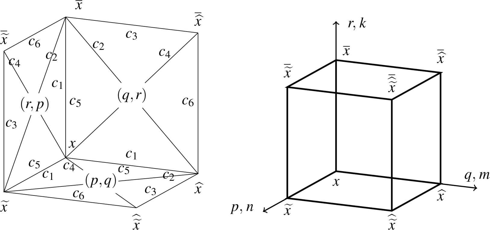
The consistency cube. The picture on the right gives the location of the variables, lattice directions and parameters. The picture on the left explains the coefficients: the variables of a product are connected by a line, adjacent to which we give the name of the corresponding coefficient function. The six functions within a quadrilateral depend on the lattice parameters given at the center of the quadrilateral.
Under the assumptions above the consistency conditions arise as follows: The equations on the faces of the consistency cube are given by:
We need precisely four initial values to compute the other values, three of the initial values should be on one quadrilateral and the fourth somewhere else. The standard way (there are others) is to take x,
1.3. Organization of the search
The condition that the different ways to compute
In analyzing the ensuing equations the solution process branches depending on whether some coefficient function is zero or not. It is not easy to keep track of such branching and therefore we choose here a different approach.
We will do a pre-analysis by setting some coefficients in (1.1) to zero. For that purpose let us write (1.1) as
With this coding the list of the 37 equations passing the conditions 1–3 of Definition 1.1 is given by
-
{5,{1,0,1,0,0,0}},{ 7,{1,1,1,0,0,0}},{10,{0,1,0,1,0,0}},{11,{1,1,0,1,0,0}},
-
{13,{1,0,1,1,0,0}},{14,{0,1,1,1,0,0}},{15,{1,1,1,1,0,0}},{21,{1,0,1,0,1,0}},
-
{23,{1,1,1,0,1,0}},{26,{0,1,0,1,1,0}},{27,{1,1,0,1,1,0}},{29,{1,0,1,1,1,0}},
-
{30,{0,1,1,1,1,0}},{31,{1,1,1,1,1,0}},{37,{1,0,1,0,0,1}},{39,{1,1,1,0,0,1}},
-
{42,{0,1,0,1,0,1}},{43,{1,1,0,1,0,1}},{45,{1,0,1,1,0,1}},{46,{0,1,1,1,0,1}},
-
{47,{1,1,1,1,0,1}},{48,{0,0,0,0,1,1}},{49,{1,0,0,0,1,1}},{50,{0,1,0,0,1,1}},
-
{51,{1,1,0,0,1,1}},{52,{0,0,1,0,1,1}},{53,{1,0,1,0,1,1}},{54,{0,1,1,0,1,1}},
-
{55,{1,1,1,0,1,1}},{56,{0,0,0,1,1,1}},{57,{1,0,0,1,1,1}},{58,{0,1,0,1,1,1}},
-
{59,{1,1,0,1,1,1}},{60,{0,0,1,1,1,1}},{61,{1,0,1,1,1,1}},{62,{0,1,1,1,1,1}},
-
{63,{1,1,1,1,1,1}}
Note that 5, 10 and 48 yield two-term equations.
In order to populate the consistency cube we need triplets of equations, leading in principle to 373 = 50653 cases, fortunately this number can be reduced by applying symmetries.
2. Symmetries
For triplets of equations we use a list {X, Y, Z} where X is the decimal code for the bottom equation, Y for the back equation and Z for the left equation. The top, front and right equations are obtained by a coordinate shift and therefore there is no need to enumerate them separately.
We will now look how some basic symmetries that do not change the CAC property operate on the codes. For easy reference we write here the triplet with ι but without lattice parameters:
2.1. Rotation
Let us first consider rotating the cube around the axis (0, 0, 0) − (1, 1, 1), counterclockwise when looking from (1, 1, 1). This moves the quadrilateral planes by (n, m) → (m, k) → (n, k) → (n, m) and certainly does not change the consistency of the equations. Thus we rotate cyclically the shifts ∼ → ^ → ¯ → ∼ accompanied with parameter change p → q → r → p. Due to the cyclic convention in writing the triplet (1.3) it means that the LHS equations become
This rotation does not change the roles of ci and therefore it corresponds to the rotation of triplet codes by
Clearly ℛ3 = 𝕀. Using rotation symmetry we can reduce the number of equation triples to be analyzed, for example if we always rotate so that X ≤ Y, Z the remaining number of cases is 17575 (in practice we use a slightly different method).
2.2. Tilde-hat reflection
In addition to rotations we need to consider some reflections. Let us first take the reflection across the plane defined by points (0, 0, 0) − (1, 1, 0) − (1, 1, 1), −(0, 0, 1), i.e. the tilde-hat reflection ∼ ↔ ^, accompanied with p ↔ q. From the point of view of the equations, this rule is all we need to know to get another triplet of CAC equations. For the search process we need to know how this and other symmetries change the triplet codes of the equations, because we need to analyze only one triplet from the orbit of a triplet.
Applying tilde-hat reflection on (2.1) we get
Comparing this with (2.1) we find that the back and left equations get exchanged, and in addition the equations change by exchanging the ι or c subscripts 1 ↔ 5 and 3 ↔ 6 (compare, e.g., (2.3c) with (2.1b)). Thus the tilde-hat reflection is given by the operator Θ
The above was for tilde-hat reflection, but we can of course also have hat-bar and bar-tilde reflections, these can be obtained using rotations: ℛΘℛ2 and ℛ2Θℛ, respectively.
We have θ2 = 𝕀 and hence Θ2 = 𝕀, furthermore ℛ2Θ = Θℛ, (Θℛ)2 = (ℛΘ)2 = 𝕀.
2.3. Tilde reversal
Another important reflection is the shift reversal. Let us consider the tilde reversal, which means reflection across the plane defined by the points
Thus for the bottom equation we have 2 ↔ 4 and 5 ↔ 6, the back equation is unchanged, and for the left equation we have 1 ↔ 3 and 2 ↔ 4. We can write the action of the reversal operation 𝒯 as
We have TaTb = TbTa,
The above was for tilde-reversal, but we can of course also have hat-reversal and bar-reversal, these can be obtained considering: ℛ𝒯ℛ2 and ℛ2𝒯ℛ.
2.4. Inversion
One important transformation that preserves affine linearity of the quad equation (up to overall factor) is the Moebius or affine linear transformation. Now that we are dealing with homogeneous equations only scaling x ↦ const. × x and inversion x ↦ 1/x remain.
From (2.1) we can read that inversion x ↦ 1/x implies 1 ↔ 3, 2 ↔ 4 and 5 ↔ 6. Similar exchanges were also seen in tilde reversal above. Indeed one finds that (ℛ𝒯)3 implies 1 ↔ 3 and 5 ↔ 6, but not 2 ↔ 4. Thus inversion would be an additional symmetry operation in cases where one of c2, c4 vanishes but not both. It will turn out that such an asymmetric possibility arises only with solutions in which c2 and c4 remain arbitrary functions, because in that case there is also solution in which one of c2, c4 vanishes. Such solutions are obtained by simple reductions and therefore we do not actually need inversion.
2.5. Orbit of the transformation group
By composing the basic operators of rotation ℛ and two reflections 𝒯 and Θ in various orders one can generate the orbit of a given initial triplet and for integrability we only need to check one representative of each orbit.
We have already mentioned some relations between the operators (and there may be others) and these can be used to eliminate some combinations as redundant. However, the full group generated by these three operations is probably rather large, but in our case we only need their representation when operating on three strings each containing six zeros or ones. It turns out that (after rotating the triplets into some canonical form) we only have orbits of length 1, 2, 4 or 8. Below we will give the orbits separately, if they have length > 1.
2.6. Gauge transformation
Finally, we can change the coefficients in the equations by a gauge transformation of the form
In order to easily check the uniformity we have introduced a fixed point n0, m0, k0, and when the gauge transformation is applied to a given equation the result cannot depend on the fixed point, except possibly through an overall multiplier. The restrictions this imposes on the parameters of the gauge transformation will depend on the particular triplet of equations.
We will use gauge transformations to simplify the final result, for example by eliminating some free coefficient(s) from the equation(s), when it simplifies the system. However, even if we can eliminate some free function ci this way, the mere possibility that such a function can exist is by itself important for classification.
3. The search
Solving the equations that result from the CAC conditions cannot be fully automatized and therefore we cannot separately solve each case of the tentative number of 17575 cases (obtained with X ≤ Y, Z). For this reason further computer scanning was done by checking whether the equations obtained from the CAC condition contain any that are monomials of the cj. Since cj are all nonzero the monomial equation cannot be satisfied and therefore that equation triplet can be omitted. This scan turned out to effective, and it was possible to analyze the remaining list of triplets (one representative per orbit).
For the triplet codes remaining after scanning we studied the equations generated by CAC until we got into a contradiction with ci ≠ 0, or one of the equations in the triplet factorized, or in the positive case, all equations were solved. The search and its results are given in A. As discussed there, we grouped the set of codes remaining after rough scanning into blocks, and only one representative of each orbit was tested. We have freely used gauge transformations (2.7) and rotations (2.2) to present the triplet equations in a nice form, for example so that the “side equations” are similar.
In the next section we group and classify the result of A.
4. Classification
The primary classification of the results is by whether or not the triplet of equations can contain free functions of two variables ci. The gauge transformation (2.7) can sometimes be used to eliminate such a function but what is relevant is whether such functions can appear (other than as overall factors).
It is also useful to observe the appearance of the c2, c4 pair, that is, terms of the type
The results we have obtained can be grouped into four sets, each set having a highest equation from which the remaining equations are obtained by reductions, possibly accompanied by rotations and reflections.
4.1. {63,10,10}
For the first group the most general triplet is
Thus the bottom equation is a completely free homogeneous quadratic equation while the side equations are simple. This is Equation (A.3) in Appendix A.1. The triply shifted x is given by
We see that this equation has the tetrahedron property if c2 = c4 = 0. The organization of the 36 sub-cases, obtained by setting some cj = 0, into orbits is given in Appendix A.2. The simplest equation in this category is (A.2) in Appendix A.1.
For {63,10,10} one cannot change the back or left equations by gauge, but as the number of terms in the bottom equation decreases there is more freedom in the side equations. This is illustrated by a CAC result in the {58,10,10} category:
It has two free functions in the back equation. However it is transformed into a sub-case of (4.1) by the gauge transformation
The possibility of extra free functions that can be gauged away is irrelevant for MDC, but they will have information value in the analysis of BTs in Section 5.4.
4.2. {10,58,15}
This triplet is Equation (A.4) in Appendix A.2. Two of the equations have four free functions each:
Note that the last two equations are not connected by a cyclic variable change but by just tilde-hat exchange (and cyclic parameter change). The triply shifted quantity is given by
The sub-cases of (4.3) are listed in Appendix A.3 and are obtainable by setting some cj = 0. For each of the four term equations there are 7 acceptable sub-cases but one of them leads to the {63,10,10} category, therefore there are 36 cases in this category. Missing cj terms sometimes allow a more general bottom equation, but that freedom can be gauged away. TET is possible only if c2(r, p) = c4(r, p) = c5(q, r) = c6(q, r) = 0 or if c1(r, p) = c3(r, p) = c2(q, r) = c4(q, r) = 0, but both reduce (4.3) to the {X,10,10} category.
4.3. {53,15,58}
Another chain of triplets that can have free functions is obtained starting with the highest equation {53,15,58} or Equation (A.11) of Appendix A.5. After a gauge transformation the result can be written as
The triply shifted variable is
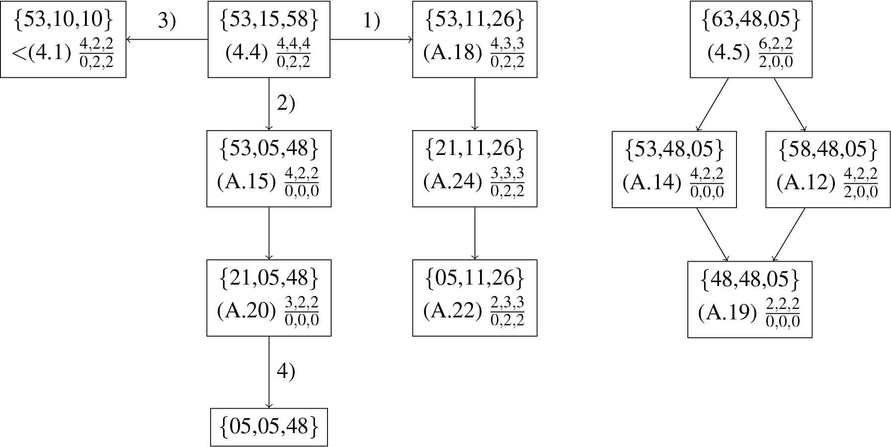
On the left some sub-case relations from {53,15,58}, on the right the reductions from {63,48,05}. Each box gives the code of the triplet and under it on the left its equation number. The ratio on the right gives above the number of terms and below the number of c2, c4 terms.
- 1)
{53,11,26} is obtained from {53,15,58} by scaling
- 2)
{53,05,48} is obtained from {53,15,58} by taking the leading term as r → ∞.
- 3)
- 4)
If in {21,05,48} we take c5 = 0, we get {05,05,48} which is rotated reflected (A.19).
4.4. {63,48,05}
Here the highest equation is Equation (A.21) of Appendix A.8:
The sign σ1 cannot be eliminated by gauge.
It has TET if c4 = 0, which has code {48,48,05}. The diagram on the RHS of Figure 2 describes the reductions of (4.5), they are all by setting some ci = 0.
4.5. {63,63,63}-2, a triplet without free functions
The highest level triplet of this set has code {63,63,63}-2, it is Equation (A.29) in Appendix. It is in fact Q3(δ = 0) of the ABS list [2]:
The triply shifted variable is
Furthermore, all other triplets that cannot have free functions are obtained by some limit from this equation. Figure 3 describes the chain of limits. From each orbit one element is mentioned and the data in the box is as in Figure 2.
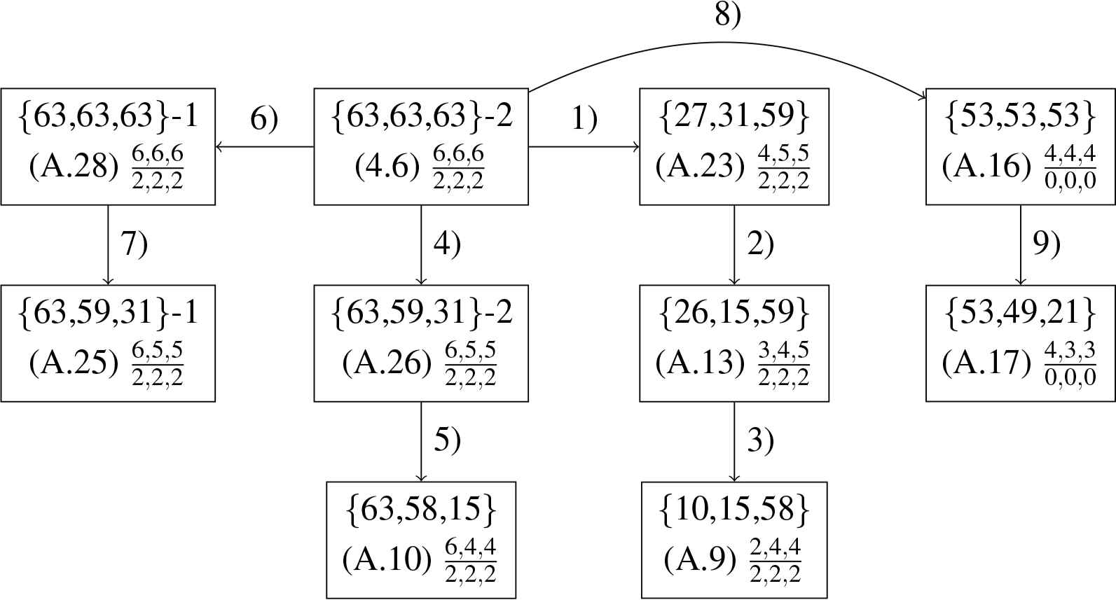
The limits given in Figure 3 are obtained as follows:
- 1)
In (4.6) scale
- 2)
In (A.23) scale
- 3)
In (A.13) scale
- 4)
In (4.6) scale
- 5)
In (A.26) scale
- 6)
In (4.6) let p ↦ 1 + εp, q ↦ 1 + εq, r ↦ 1 + εr and take the leading term as ε → 0.
- 7)
In (A.28) scale
- 8)
In (4.6) take the leading term (linear) as p, q, r → 0.
- 9)
In (A.16) scale
In this way all equations to which free functions of two variables cannot be introduced by a gauge are reductions of Q3(δ = 0) (4.6).
It should be noted, however, that in Figure 3 the bottom box {10,15,58} (A.9) is an equation that does allow free functions, and this happens also on further reductions from the other bottom boxes: From {63,58,15} (A.10) the limit p, q → 0 leads to {53,10,10} while p, q → ∞ leads to {53,48,05} (A.14); from {10,15,58} (A.9) the limit r → leads to {10,05,10} while r → ∞ leads to {10,10,48}, which are in the same orbit; from {53,49,21} (A.17) the limit p, q → ∞ leads to {53,48,05} (A.14). All of these further limits yield equations which allow free functions. It should be noted also that some potential limits actually lead to factorizable equations, for example if in {63,59,31}-1 (A.25) one takes p, q → 0 or if in {63,58,15} (A.10) one takes p ↦ 1 + εp, q ↦ 1 + εq, r ↦ 1 + εr and then take the leading term as ε → 0.
We also note that (4.6) still allows gauge transformations of the form
4.6. Comparison with Boll’s results
As was mentioned before, Boll has done a classification of triplets of CAC equations in [3–5]. His setup was both more general (allowing flips between opposing sides and not restricting to homogeneous quadratic equations) and less general (by requiring the tetrahedron property). In [3] the results were collected into Theorems 3.4–3.11. Restricting those equations to quadratic irreducible equations without flips implies some restrictions on the parameters, and yield the following:
- 1)
- 2)
- 3)
- 4)
- 5)
- 6)
- 7)
- 8)
For (3.33–34) we must take δ1 = 0, then it gives reflected (A.18). In B all coefficients can be free.
- 9)
- 10)
For (3.43–44) we must take δ1 = δ2 = 0, then it becomes rotated form of (A.20). (Note that in the formula for C the first variable must be x13, not x12.)
Thus all homogeneous quadratic shift invariant equations in Boll’s classification [3] are also included in our classification. However, there is one result we could not identify among Boll’s results, namely (A.25), which is related to Q1 the same way that (A.26) is related to Q3, and (A.16) is related to H3.
4.7. Triplets with two term equations
As another selection of our results we would like to collect here the simplest CAC triplets, those for which all equations have just two terms. Below on the LHS they are given in the general form after all equations from the CAC condition have been solved, and then on the RHS we present the simplest form obtainable by a gauge transform.
-
{10,10,10}
-
{5,10,10} or {48,10,10} by tilde-hat reflection
-
{10,48,5}
-
{5,5,48} and {48,5,48} by tilde-hat reflection
These cases are easily distinguished by the number of c2, c4 terms, which have also been rotated into a particular position. These triplets can be obtained from several results listed in the Appendix by various limits.
Summary
The triplets that were found using CAC can be divided into two groups: 1) Those that cannot have free functions of two lattice parameters are all reductions of Q3(δ = 0) of the ABS list [2]. 2) The triplets that can have free functions of two lattice parameters can be organized into 4 sets, with the highest triplets of the set being {63,10,10}, {53,15,58}, {63,48,05}, or {10,58,15}.
5. Bäcklund transformations and Lax pairs
The equations that were found using CAC will next be studied from the point of view of their Bäcklund transformations and Lax pairs.
5.1. General setup
Let us fix the equations and some concepts. We have six equations, which we can arrange as follows:
This is the same set as (1.3), except that we have named
Definition 5.1 (Bäcklund transform of equations (eqBT)).
Consider equations (5.1b) and (5.1c) and solve for ŷ and ỹ from their LHS. Then from the RHS of these equations we can solve for
Note that if the system (5.1) has the CAC property then the above mentioned two results for
Definition 5.2 (Bäcklund transform of solutions (solBT)).
Suppose x is a solution of (5.1d). If we can solve for y from (5.1b) and (5.1c) and that solution solves (5.1a) then we have a BT transforming solutions. If x = y then the transformation is trivial.
Since we are only interested in the equations and their relationships we only use eqBT as described in Definition 5.1.
Before doing any computations we can already make some statements about the triplets that we have found. The starting setup was that all coefficients in the triplet of equations were free functions depending on the two lattice parameters associated with that quadrilateral, and then from the CAC we got conditions due to which some two-variable functions were fixed. However, we have seen that sometimes even if a triplet is CAC it may still contain arbitrary functions ci (other than overall factors).
If we now look at this from the point of view of eqBT, it is clear that an equation with a free function cannot be generated by an eqBT composed of the remaining pair of equations, because of different dependence on lattice parameters. For example, when the side equations only contain cj(q, r) and cj(r, p) they cannot be used to construct arbitrary free cj(p, q). Furthermore, since gauge transformations have no effect on the eqBT, it turns out that the important property is the possibility of free functions (other than overall multipliers). For example for (A.2) BT produces nothing and this can be predicted from the fact that by gauge freedom each equation can have free functions as shown in (A.1). In the case of the triplet (4.2) the bottom and back equations may contain free functions and therefore a eqBT can at most produce the back equation.
In comparing eqBT and CAC we note that for CAC there is no fundamental difference in the roles of the equations, while for eqBT the middle equations (5.1b), (5.1c) form the transformation using which we should be able to generate top and bottom equations. In a closer analysis we observe that for CAC and eqBT the computations start the same way: If we take x,
-
In the next step for CAC we would solve for
-
In eqBT we are only working with Q23 and Q31, and therefore only have the front equation remaining. It should now factorize with one factor being the bottom equation, the other factor possibly containing y.
In practice the methods differ when the front equation vanishes before substituting
We note also that in (5.1) the roles of x and y are symmetric and therefore the same arguments can be used to generate the top equation. Furthermore, if we instead rename
5.2. Computations for eqBT
In order to further analyze the eqBT, it is useful to develop the formulae to some extent without specifying the form of the Q-polynomials. For this purpose it is often useful to isolate one of the variables of Q, but since Q is multilinear this is easy. We can write, for example,
Using this notation we can solve the LHS equations of (5.1b), (5.1c),
Let us furthermore expand these in y since it cannot appear in final equation. We have
We use the symbol ≗ for equalities that should hold modulo an acceptable equation. For a set of equations the equality should be modulo the same equation, which we call Q12.
Since Q12 does not contain y, the Bäcklund condition
For a genuine eqBT these equations should not all be satisfied automatically but rather for at least one equation the LHS should factor with an acceptable equation as a factor.
5.3. Deriving the Lax condition
It is interesting to compare eqBT with conditions derived from a Lax pair. The starting point is still (5.2), but now we replace y → f/g. Thus for example
Then the commutativity condition
The entries of this matrix equation are
These equations should either vanish, or factorize with the desired equation as a factor.
When comparing (5.8) with (5.5) it is easy to verify that (5.8) implies (5.5). However, in the other direction one finds that in addition to
5.4. BT for the results obtained
Above we have described how the eqBT computations lead to equations (5.5) which should not hold automatically, but only after using Q12 = 0, in other words,
- (1)
back-left-front-right equations producing bottom and top equations,
- (2)
bottom-back-top-front equations producing left and right equations,
- (3)
bottom-left-top-right equations producing back and front equation.
We have done these computations for all equations found to have CAC (one representative per orbit) as listed in A. The results are given in Tables 1–3. In the table a “0” means the corresponding eqBT produces nothing, i.e., the equations (5.5) are satisfied automatically, a “1” means the desired equation is uniquely produced. The remaining cases have a “2” indicating that the polynomial produced by the BT has two factors that can be taken as genuine equations (i.e. they are acceptable by Definition 1.1 and do not depend on the auxiliary variable y). A plain “2” means the two possibilities differ only by a sign, “2cn” means that the extra equation has degree n dependence on the cj, while 2* stands for the cases where the two equations are essentially different and the extra equation is a version of
| Eqn | Top | Bottom | Left | Right | Back | Front | TET |
|---|---|---|---|---|---|---|---|
| 63,10,10 | 0 | 0 | 1 | 1 | 1 | 1 | no |
| 62,10,10 | 0 | 0 | 1 | 1 | 1 | 1 | no |
| 58,10,10 | 0 | 0 | 2c2 | 2c2 | 0 | 0 | no |
| 42,10,10 | 0 | 0 | 1 | 1 | 0 | 0 | no |
| 10,10,10 | 0 | 0 | 0 | 0 | 0 | 0 | no |
|
|
|||||||
| 43,10,10 | 0 | 0 | 1 | 1 | 1 | 1 | no |
|
|
|||||||
| 61,10,10 | 0 | 0 | 1 | 1 | 1 | 1 | no |
| 60,10,10 | 0 | 0 | 1 | 1 | 1 | 1 | no |
| 56,10,10 | 0 | 0 | 2c1 | 2c1 | 0 | 0 | no |
|
|
|||||||
| 53,10,10 | 0 | 0 | 1 | 1 | 1 | 1 | yes |
| 52,10,10 | 0 | 0 | 1 | 1 | 1 | 1 | yes |
| 05,10,10 | 0 | 0 | 0 | 0 | 2 | 2 | yes |
Results of eqBT for two classes of equations that can have free functions. “2” in a column means BT produces two possibilities, “2cn” that the non-standard alternative has polynomial coefficients of degree n in ci. Only one representative of each orbit is listed. In the last column we indicate whether the triplet has the tetrahedron property.
(a) eqBT for equations of type {X,10,10}.
| Eqn | Top | Bottom | Left | Right | Back | Front | TET |
|---|---|---|---|---|---|---|---|
| 10,58,15 | 2c4 | 2c4 | 0 | 0 | 0 | 0 | no |
| 10,58,07 | 2c3 | 2c3 | 0 | 0 | 0 | 0 | no |
| 10,58,11 | 2c3 | 2c3 | 0 | 0 | 0 | 0 | no |
| 10,26,11 | 1 | 1 | 0 | 0 | 0 | 0 | no |
| 10,50,11 | 2c2 | 2c2 | 0 | 0 | 0 | 0 | no |
| 10,50,07 | 1 | 1 | 0 | 0 | 0 | 0 | no |
| 10,58,05 | 2c2 | 2c2 | 0 | 0 | 0 | 0 | no |
| 10,56,05 | 1 | 1 | 0 | 0 | 0 | 0 | no |
| 10,26,05 | 2c1 | 2c1 | 0 | 0 | 0 | 0 | no |
| 10,48,05 | 0 | 0 | 0 | 0 | 0 | 0 | no |
(b) eqBT for sub-cases of {10,58,15}.
| Eqn | Top | Bottom | Left | Right | Back | Front | TET |
|---|---|---|---|---|---|---|---|
| 53,15,58 (4.4) | 0 | 0 | 1 | 1 | 1 | 1 | yes |
| 53,05,48 (A.15) | 0 | 0 | 1 | 1 | 1 | 1 | yes |
| 21,05,48 (A.20) | 0 | 0 | 1 | 1 | 1 | 1 | yes |
|
|
|||||||
| 53,11,26 (A.18) | 0 | 0 | 1 | 1 | 1 | 1 | yes |
| 21,11,26 (A.24) | 0 | 0 | 1 | 1 | 1 | 1 | yes |
| 05,11,26 (A.22) | 0 | 0 | 1 | 1 | 2* | 2* | yes |
|
|
|||||||
| 63,48,05 (4.5) | 0 | 0 | 1 | 1 | 1 | 1 | no |
| 58,48,05 (A.12) | 0 | 0 | 2c1 | 2c1 | 0 | 0 | no |
| 53,48,05 (A.14) | 0 | 0 | 1 | 1 | 1 | 1 | yes |
| 48,48,05 (A.19) | 0 | 0 | 2 | 2 | 0 | 0 | yes |
|
|
|||||||
| 10,15,58 (A.9) | 0 | 0 | 2* | 2* | 2* | 2* | yes |
eqBT for triplets with arbitrary functions listed in Figure 2.
| Eqn | Top | Bottom | Left | Right | Back | Front | param |
|---|---|---|---|---|---|---|---|
| 63,63,63-1 (A.28) | 1 | 1 | 1 | 1 | 1 | 1 | p, q, r |
| 63,59,31-1 (A.25) | 23 | 21 | 1 | 1 | 1 | 1 | p, q |
|
|
|||||||
| 63,63,63-2 (4.6) | 1 | 1 | 1 | 1 | 1 | 1 | p, q, r |
| 63,59,31-2 (A.26) | 1 | 1 | 1 | 1 | 1 | 1 | p, q |
| 63,58,15 (A.10) | 2* | 2* | 1 | 1 | 1 | 1 | p, q |
|
|
|||||||
| 27,31,59 (A.23) | 1 | 1 | 1 | 1 | 1 | 1 | r |
| 26,15,59 (A.13) | 1 | 1 | 2* | 2* | 1 | 1 | r |
| 10,15,58 (A.9) | 0 | 0 | 2* | 2* | 2* | 2* | r |
|
|
|||||||
| 53,53,53 (A.16) | 1 | 1 | 1 | 1 | 1 | 1 | p, q, r |
| 53,49,21 (A.17) | 1 | 1 | 1 | 1 | 1 | 1 | p, q |
eqBT for triplets in Figure 3, with specific p, q, r dependency listed. As mentioned they are all reductions of {63,63,63–2}. For {63,59,31}-1 the subscript gives the degree of the other equation. All of these equations have the tetrahedron property. Note that the reduction{10,15,58} can have free ci functions and therefore it fails some eqBTs, which is indicated by the 0 entries.
Here are some examples
-
For equation {58,10,10} the bottom-back-top-front side equations produce for the left equation a rational expression whose numerator factorizes as
-
The factor in round brackets is the expected left equation. Note that for the alternate equation in square brackets the q dependence is superfluous since the back equation should only depend on r, p.
-
For equation {10,15,58} the the bottom-back-top-front side equations produce
-
The term in square brackets is the proper left equation, the extra factor
-
For {63,59,31}-1 eqBT produces the bottom equation and as an alternative,
Summary
All the equations discussed here satisfy the consistency-around-the-cube condition. The equations on the consistency cube can also provide a Lax pair or produce a Bäcklund transformation in which the “side equations” may generate the bottom and top equations. It turns out that many of the equations produce a fake Lax pair or equivalently an empty eqBT. From the tables we can also read that some equations have the tetrahedron property and still fail with respect to eqBT. Furthermore some equations have ambiguous eqBT, generating two possible equations. If such a triplet does not completely fail in any direction we may have an example of partial integrability.
6. Discussion
We have searched for all homogeneous quadratic triplets of multilinear irreducible equations that satisfy the Consistency-Around-a-Cube condition with uniform embedding (translation invariance of quad equations). The results were given in A and classified in Section 4. The three equations forming the triplet were allowed to have different forms, while in the usual setup the bottom equation is given and the other equations are obtained from that by definite variable and parameter changes. In that sense our approach is close to that of Boll [3, 5].
The ansatz for the equations contained coefficients that depended on the two lattice parameters associated with the quadrilateral in question. The results can be divided into two classes: those that cannot have arbitrary dependence on the two lattice parameters and those that can. The arbitrary functions can sometimes be eliminated by a gauge transformation (that preserves uniformity) and therefore the possibility of free functions is essential. The results can be arranged into sub-cases, some relations are given in Figures 2–3. The equations that cannot have free functions are all reductions of Q3(δ = 0) of the ABS list [2].
Recently it has been noted that some equations that pass the CAC test can have fake Lax pairs [6], and independently the possibility of “weak Lax pairs” has also been observed [8]. In order to characterize the equations further we studied how the Bäcklund transformation works on these equations. The result are given in Tables 1–3. One finds that all equations that can have free functions also have some failing BTs (or equivalently some fake Lax pairs). This is natural since it is not possible to generate a free function from equations that do not contain them. Note that some of the equations with failing eqBTs do nevertheless have the tetrahedron property.
From our results we infer the following:
- (1)
The CAC condition can only be a necessary condition of integrability. It cannot be sufficient as many equations with failing eqBTs pass this test.
- (2)
The CAC condition may be sufficient if accompanied with some other type of condition, but the tetrahedron condition is not enough for that purpose.
- (3)
We conjecture that if there is a unique BT for each direction of the cube then that should be sufficient for integrability. Non-uniqueness in some directions may be a signal of partial integrability while failure of the BT in one or more directions suggests non-integrability.
- (4)
Integrability may be lost during reductions. But note that the reduction here does not change dimension but just means simplifying the equation by some limit of the coefficient(s).
A. Results of the search
We will now list the CAC equation triplets within the category of equations studied in this paper, namely those that are quadratic and acceptable by Definition 1.1. We list them following the order of the search process which was based on the triplet code. In Section 4 they are grouped according to the “highest equation” and its reductions. During the search process sub-case inclusion was not considered except for obvious reductions. If the triplet found is a member of a symmetry orbit of more than one entry we also list the orbit.
A.1. {10,10,10}
The triplet
A.2. {X,10,10}, X ≠ 10
This category contains the triplet {63,10,10} and its special cases.
That is, a completely arbitrary homogeneous quadratic equation is MDC with the side equations as given above. The triply shifted x is given by
The sub-cases of {63,10,10} arrange themselves into orbits as follows:
-
6 terms: {63,10,10}
-
5 terms: {55,10,10},{61,10,10},
-
5 terms: {31,10,10},{47,10,10},{59,10,10},{62,10,10}
-
4 terms: {53,10,10},
-
4 terms: {15,10,10},{58,10,10},
-
4 terms: {27,10,10},{30,10,10},{43,10,10},{46,10,10},
-
4 terms: {23,10,10},{45,10,10},{29,10,10},{51,10,10},{57,10,10}, {60,10,10},{39,10,10},{54,10,10},
-
3 terms: {7,10,10},{13,10,10},{50,10,10},{56,10,10},
-
3 terms: {11,10,10},{14,10,10},{26,10,10},{42,10,10},
-
3 terms: {21,10,10},{37,10,10},{49,10,10},{52,10,10},
-
2 terms: {5,10,10},{48,10,10}.
In solving the CAC equations for these triplet codes we were usually led to conditions on the c2, c4 terms of the back and left equation. For {63,10,10} it is not possible to have any free functions in the side equations, but as the {58,10,10} (4.2) case shows, with smaller number of terms in the bottom equation we have more freedom in the side equations but that freedom can be eliminated by gauge.
A.3. {10,X,Y}, X,Y ≠ 10
In this case we arrange the bottom equation to be the simple one. The main result in this category is {10,58,15}:
The triply shifted quantity is given by
This has sub-cases when one or two ci in either or both equations vanish while keeping the equations irreducible. Missing cj terms sometimes allow a more general bottom equation, but that freedom can be gauged away. The sub-case orbits are as follows:
-
2,4,4 terms: {10,58,15},
-
2,3,4 terms: {10,58,7},{10,58,13},{10,50,15},{10,56,15},
-
2,3,4 terms: {10,58,11},{10,58,14},{10,26,15},{10,42,15},
-
2,3,3 terms: {10,26,11},{10,26,14},{10,42,11},{10,42,14},
-
2,3,3 terms: {10,50,11},{10,50,14},{10,56,11},{10,26,7},{10,26,13}, {10,42,7}, {10,56,14},{10,42,13},
-
2,3,3 terms: {10,50,7},{10,50,13},{10,56,13},{10,56,7},
-
2,2,4 terms: {10,58,5},{10,48,15},
-
2,2,3 terms: {10,56,5},{10,50,5},{10,48,13},{10,48,7},
-
2,2,3 terms: {10,26,5},{10,42,5},{10,48,11},{10,48,14},
-
2,2,2 terms: {10,48,5}.
The number of terms in each equation is given in the first column, but that list is not ordered because some reflections exchange back and left equations. The sub-cases belonging to {X,10,10} are excluded.
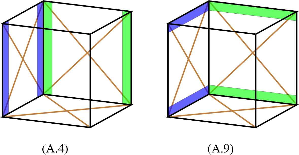
{10, 15, 58} In this category there is also an equation that is not a sub-case of (A.4):
This cannot be a sub-case of (4.3) because the equations do not contain the same shifted x variables. We can use gauge transformation to simplify this further. Choosing the gauge so that (A.7) simplifies to
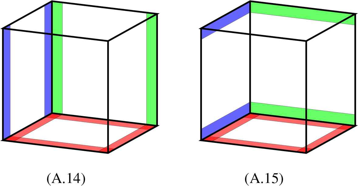
For an intuitive understanding of the difference between (A.4) and (A.9) we can look at the Figure 4. Note also that in (A.5) x̄ is in the numerator while in (A.8) it is in the denominator.
A.4. {58, 15, X}, X ≠ 10
Only {63,58,15} survives, all other cases lead to equations that factorize.
A.5. {15, 58, X}, X ≠ 10, 15, 58
According to (2.4a) we have by tilde-hat reflection and rotation {15,58,X} → {58,θX,15} → {15,58,θX}. Thus {15,58,X} and {58,15,Y}, are not related by this reflection and may have different types of solutions.
The main solution in this category is {53,15,58}, and after a gauge transformation the equation satisfying CAC can be written as
The triply shifted variable is
-
4 terms: {53,15,58},
-
3 terms: {21,15,58},{37,15,58},{49,15,58},{52,15,58},
-
2 terms: {5,15,58},{48,15,58}.
A.6. {15, X, Y}, X, Y ∉ {10, 58} or {58, X, Y}, X, Y ∉ {10, 15}
By the tilde-hat reflection we have {15,X,Y} → {58, θY, θX} and therefore there is one-to-one correspondence between the sets {15, X, Y} and {58, X′, Y′} and we only need to discuss one of them.
There are types two solutions, the first one is {58,48,5} given by
One can change some of the signs by gauge but one cannot eliminate the freedom in ci. This does not have TET except if c4(p, q) = 0, in which case it becomes {48,48,5} (A.19). The reflected case is {15,48,5}.
{26,15,59} The second solution is, after gauge and rotation
The triplet (A.13) is symmetric under bar reversal and tilde reversal, but not under hat-reversal and therefore there are also the corresponding solutions within three reversed categories. The orbit is {15,59,26},{15,62,42},{58,11,31},{58,14,47}.
A.7. {53, X, Y}, X,Y ∉ {10, 15, 58}
There are five solutions in this category and they all have TET.
{53,48,5}
{53,5,48}
The sub-case orbits are as for {53,15,58} (A.11).
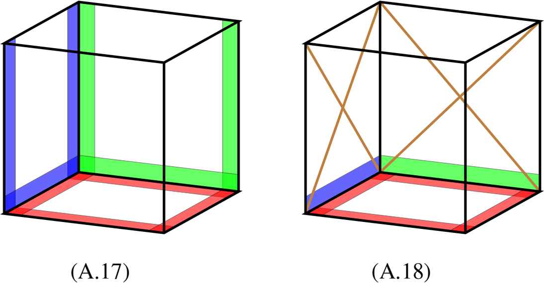
The difference between (A.14) and (A.15) is illustrated in Figure 5.
{53,53,53}
We have added here some coefficients δα and ρα and if they are nonzero they can be gauged to 1, which yields H3(δ = 0) of the ABS list. If a ρα vanishes we get a rotation of {53,49,21}, if a δα vanishes we get a rotation of its reflection {53,52,37}, and if δα = ρα = 0 for some α we get a rotation of a special case of {53,48,05}.
{53,49,21}
There is also the reflected case {53,52,37}.
{53,11,26}
Note that
The difference between (A.17) and (A.18) is illustrated in Figure 6.
A.8. {5, X, Y } or {48, X, Y}X, Y ∉ {10, 15, 53, 58}
By the tilde-hat reflection we have {5, X, Y} → {48, θY, θX}. The solutions in this category are as follows:
{48,48,05}
The signs can be controlled by gauge. In this orbit there is also {05,05,48}.
{21,05,48}
The full orbit of reflected cases is {21,5,48}, {37,5,48}, {49,5,48}, {52,5,48}.
{63,48,5}
The sign σ1 cannot be eliminated by gauge.
{5,11,26}
The orbit is {5,11,26}, {48,11,26}, {5,14,42}, {48,14,42}.
A.9. The rest:{X, Y, Z}, X, Y, Z ∉ {5, 10, 15, 53, 58}
{27,31,59}
There are altogether 4 different reflections of this triplet: {27,31,59}, {43,31,62}, {30,47,59}, {46,47,62}.
{21,11,26}
There are 8 elements in the orbit {11,26,21}, {11,26,37}, {11,26,49}, {11,26,52}, {14,42,21}, {14,42,37}, {14,42,49}, {14,42,52};
The remaining cases were the difficult ones to solve. In the category {63,59,31} there are two solutions:
{63,59,31}-1
Note that the back and left equations are not related by a cyclic variable change.
{63,59,31}-2
There are also corresponding two reflected cases {63,62,47}.
{63,63,63} In the category {63,63,63} there are also two solutions. The preliminary way of writing the result, after a gauge transformation, is the form
If a1 and/or a0 are nonzero the result is awkward, but we can simplify the result by a transformation p = f(P), q = f(Q), r = f(R). However, in order to connect with known results we want the coefficient of the
{63,63,63}-1 If a2 = 0 then by a simple translation we get c(α) = ε(α)α, where ε(α)2 = 1, but this sign can be eliminated by gauge. In order to connect with known results we redefine p ↦ 1/p, q ↦ 1/q, r ↦ 1/r after which we get
This is in fact Q1(δ = 0) in the ABS list.
{63,63,63}-2 A different solution is obtained if a2 ≠ 0. Then by transforming
Note that the difference between Q1 and Q3 arises from the factorization properties of the c(α) coefficient in (A.27).
Acknowledgment
I would like to thank Da-jun Zhang for useful comments on the manuscript. All computations were done using the REDUCE computer algebra system [7].
Footnotes
For example the existence of N-soliton solutions for (1 + 1) dimensional PDE’s is strongly associated with integrability, but it does not even make sense for Hamiltonian mechanical systems.
References
Cite this article
TY  - JOUR
AU  - Jarmo Hietarinta
PY  - 2021
DA  - 2021/01/06
TI  - Search for CAC-integrable homogeneous quadratic triplets of quad equations and their classification by BT and Lax
JO  - Journal of Nonlinear Mathematical Physics
SP  - 358
EP  - 389
VL  - 26
IS  - 3
SN  - 1776-0852
UR  - https://doi.org/10.1080/14029251.2019.1613047
DO  - 10.1080/14029251.2019.1613047
ID  - Hietarinta2021
ER  -