
The Riemann–Hilbert problem to coupled nonlinear Schrödinger equation: Long-time dynamics on the half-line
- DOI
- 10.1080/14029251.2019.1613055How to use a DOI?
- Keywords
- Coupled nonlinear Schrödinger equation; Riemann–Hilbert problem; Initial-boundary value problem; Long-time asymptotics
- Abstract
We derive the long-time asymptotics for the solution of initial-boundary value problem of coupled nonlinear Schrödinger equation whose Lax pair involves 3 × 3 matrix in present paper. Based on a nonlinear steepest descent analysis of an associated 3 × 3 matrix Riemann–Hilbert problem, we can give the precise asymptotic formulas for the solution of the coupled nonlinear Schrödinger equation on the half-line.
- Copyright
- © 2019 The Authors. Published by Atlantis and Taylor & Francis
- Open Access
- This is an open access article distributed under the CC BY-NC 4.0 license (http://creativecommons.org/licenses/by-nc/4.0/).
1. Introduction
The well-known nonlinear steepest descent method first introduced by Deift and Zhou in [14] provides a powerful technique for determining asymptotics of solutions of nonlinear integrable evolution equations. This approach since then has been successfully applied in analyzing the long-time asymptotics of initial-value problems (IVPs) for a number of nonlinear integrable partial differential equations (PDEs) associated with 2 × 2 matrix spectral problems including the modified Kortewegde Vries (mKdV) equation [14], the defocusing nonlinear Schrödinger (NLS) equation [15], the KdV equation [19], the derivative NLS equation [25], the Fokas–Lenells equation [28], the short pulse equation [10] and the Kundu–Eckhaus equation [27]. Moreover, by combining the ideas of [14] with the so-called “g-function mechanism” [13], it is also possible to study asymptotics of solutions of the IVPs with shock-type oscillating initial data [11], nondecaying step-like initial data [6,22], nonzero boundary conditions at infinity [4] for various integrable equations. There also exists some meaningful papers [8, 9, 17] about the study of long-time asymptotics for the IVPs of integrable nonlinear evolution equations associated with 3 × 3 matrix spectral problems. For the large-time asymptotic analysis of the initial-boundary value problems (IBVPs) of integrable nonlinear PDEs, Lenells et al. derived some interesting asymptotic formulas for the solutions of mKdV equation [23] and derivative NLS equation [3] by using the steepest descent method. Furthermore, the long-time asymptotics for the focusing NLS equation with t-periodic boundary condition on the half-line is analyzed in [5]. We also have done some work about determining the long-time asymptotics for integrable equations on the half-line, see [20, 21]. However, there is only a little of literature [7] to consider the asymptotic behaviors for integrable nonlinear PDEs with Lax pairs involving 3 × 3 matrices on the half-line. Thus, it is necessary and important to consider the large-time asymptotic behaviors for the IBVPs of integrable equations with 3 × 3 Lax pairs on the half-line.
In particular, the purpose of this paper is aim to consider the long-time asymptotics for the IBVP of the coupled nonlinear Schrödinger (CNLS) equation
We will denote the initial data, Dirichlet and Neumann boundary values of (1.1) as follows:
We also suppose that {u0(x), v0(x)} and
Our goal here is to derive the long-time asymptotics of the solution of (1.1) on the half-line by performing a nonlinear steepest descent analysis of the associated RH problem. Compared with other integrable equations, the asymptotic analysis of (1.1) presents some distinctive features: (1) Since the RH problem associated with (1.1) involves 3 × 3 jump matrix J(x, t, k), we first introduce two 2 × 1 vector-valued spectral functions r1(k), h(k) and a 1 × 2 vector-valued spectral function r(k), and then rewrite our main RH problem as a 2 × 2 block one. This procedure is more convenient for the following long-time asymptotic analysis. (2) As we all known, the important step of the steepest descent method is to split the jump matrix J(x, t, k) into an appropriate upper/lower triangular form. This immediately leads to construct a δ(k) function to remove the middle matrix term, however, the function δ satisfies a 2 × 2 matrix RH problem in our present problem. The unsolvability of the 2 × 2 matrix function δ(k) is a challenge when we perform the scaling transformation to reduce the RH problem to a model RH problem. Fortunately, we can follow the idea introduced in [18] to use the available function detδ(k) which can be explicitly solved by the Plemelj formula to approximate the function δ(k) by error control. (3) The relevant RH problem for the Cauchy problem (1.1) considered in [17] only has a jump across ℝ, whereas the RH problem for the IBVP also has a jump across iℝ, and the jump across this line involves the spectral function h(k). Moreover, during the asymptotic analysis, one should find an analytic approximation ha(t, k) of h(k). (4) Recalling the meaningful work about analyzing the long-time asymptotics for the Degasperis–Procesi equation on the half-line, the analysis presented in [7] shows that the structure of the jump matrix, which is 3 × 3, is essentially 2 × 2 (under an appropriate change of basis), whereas the analysis given in our present paper is more general.
The main result of this paper is stated as the following theorem.
Theorem 1.1.
Assume the assumption 1 be valid. Then, for any positive constant N, as t → ∞, the solution (u(x, t) v(x, t)) of the IBVP for the CNLS equation (1.1) on the half-line satisfies the following asymptotic formula
Remark 1.1.
The asymptotic formula for the half-line problem obtained in Theorem 1.1 has the exact same functional form for the pure initial value problem. The only difference is that the definition of the spectral function r(k) for the half-line problem, which enters the asymptotic formula, involves not only the initial data but also the boundary values. In other words, the only effect of the boundary is to modify r(k). We can understand this as follows: since x grows faster than t in the given region, the distance to the boundary eventually gets so big that what happens at the boundary has a small effect on the solution (recall that we assume that the boundary values decay as t → ∞). Therefore, the boundary values and the initial data play similar roles and it is natural that they enter the asymptotic formula in similar ways.
The outline of the paper is following. In Section 2, we recall how the solution of CNLS equation (1.1) on the half-line can be expressed in terms of the solution of a 3 × 3 matrix RH problem. In section 3, we present the detailed derivation of the long-time asymptotics for the solution of CNLS equation, that is, we prove Theorem 1.1.
2. Preliminaries
In this section, we give a short review of the RH problem for (1.1) on the half-line, see [18] for further details. The Lax pair of equation (1.1) is
Let
We define the matrix-valued spectral functions s(k) and S(k) by the relations
Evaluation of (2.7) at (x, t) = (0, 0) gives the following expressions
Hence, the functions s(k) and S(k) can be obtained respectively from the evaluations at x = 0 and at t = 0 of the functions μ3(x, 0, k) and μ1(0, t, k).
On the other hand, we can deduce from the properties of μj that s(k) and S(k) have the following properties:
- (i)
s(k) is bounded and analytic for k ∈ (D3 ∪ D4, D1 ∪ D2,D1 ∪ D2), S(k) is bounded and analytic for k ∈ (D2 ∪ D4, D1 ∪ D3, D1 ∪ D3);
- (ii)
dets(k) = 1 for k ∈ ℝ, detS(k) = 1 for k ∈ ℝ ∪ iℝ;
- (iii)
s(k) = I + O(k−1) and S(k) = I + O(k−1) uniformly as k → ∞;
- (iv)where
The initial and boundary values of a solution of the CNLS equation (1.1) are not independent. It turns out that the spectral functions s(k) and S(k) must satisfy a surprisingly simple relation
For each n = 1,...,4, we define solution Mn(x, t, k) of (2.1) by the solution of following Fredholm integral equation:
According to (2.11), the
Then, equation (2.13) can be rewritten in the form of a 3 × 3 RH problem as follows:
The contour for this RH problem is depicted in Fig. 1.
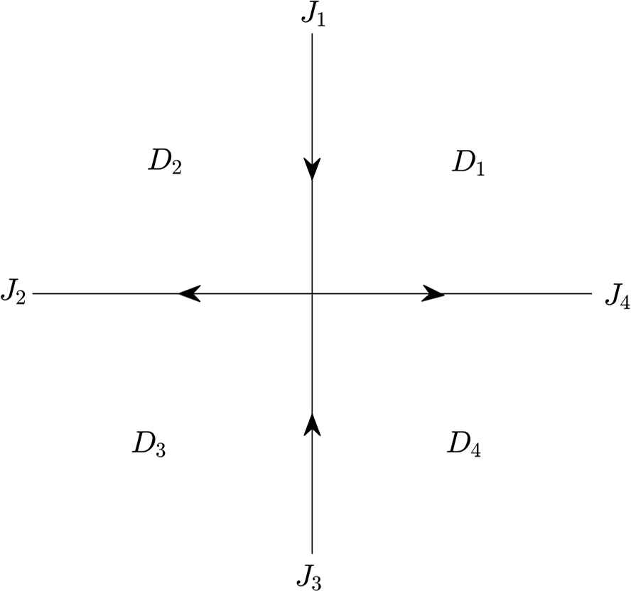
The contour for the RH problem.
In what follows, we will make the following simple assumptions.
Assumption 1. We assume that the following conditions hold:
-
the initial and boundary values lie in the Schwartz class.
-
the spectral functions s(k), S(k) defined in (2.7) satisfy the global relation (2.10).
-
s11(k) and W11(k) have no zeros in
-
all the initial and boundary values are compatible with equation (1.1) to all orders at x = t = 0.
We have the following representation theorem (the proof can be found in [18]).
Theorem 2.1.
Let u0(x), g0(t), g1(t), v0(x), h0(t), h1(t) be functions in the Schwartz class 𝒮([0, ∞)), and the assumption 1 is satisfied. Then the RH problem (2.14) with the jump matrices given by (2.15) and the following asymptotics:
Then {u(x, t), v(x, t)} satisfies the CNLS equation (1.1). Furthermore, {u(x, t), v(x, t)} satisfies the initial and boundary value conditions
Remark 2.1.
In the case when s11(k) and W11(k) have no zeros, the unique solvability of above RH problem (2.14) is a consequence of the ‘vanishing’ lemma (the proof can be found in the appendix of [18]).
Remark 2.2.
For a well-posed problem, only a subset of the initial and boundary values can be independently prescribed. However, all boundary values are needed for the definition of S(k), and hence for the formulation of the main RH problem as well as the spectral function r(k) defined in (3.3). In general, the computation of the unknown boundary values, namely, the construction of the generalized Dirichlet-to-Neumann map, involves the solution of a nonlinear Volterra integral equation. We do not consider this parts in present paper since the detailed analysis has been studied in the paper [18], (see the Sections 5 and 6 in [18]). Our main concern in present paper is the derivation of the long-time asymptotics for the solution of the IBVP of the CNLS equation (1.1).
3. Long-time asymptotic analysis
Before we proceed to the following analysis, we will follow the ideas used in [2, 17] to rewrite our main 3 × 3 matrix RH problem as a 2 × 2 block one. This procedure is more convenient for the following long-time asymptotic analysis. More precisely, we rewrite a 3 × 3 matrix A as a block form
Then we can rewrite the RH problem (2.14) as
Moreover, we can deduce from the properties of s(k) and S(k) that the functions r1(k), h(k), r(k) defined by (3.1), (3.2) and (3.3) possess the following properties:
-
r1(k) is smooth and bounded on ℝ;
-
h(k) is smooth and bounded on
-
r(k) is smooth and bounded on ℝ−;
-
There exist complex constants
3.1. Transformations of the RH problem
Let N > 1 be given, and let ℐ denote the interval ℐ = (0, N]. The jump matrix J defined in (3.5) involves the exponentials e±tΦ. It follows that there is a single stationary point located at the point where
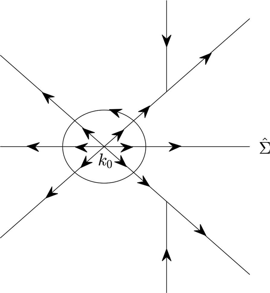
The first transformation is to deform the vertical part of Σ so that it passes through the critical point k0. Letting U1 and U2 denote the triangular domains shown in Fig. 2. Then the first transform is as follows:
The contour Σ(1) in the complex k-plane.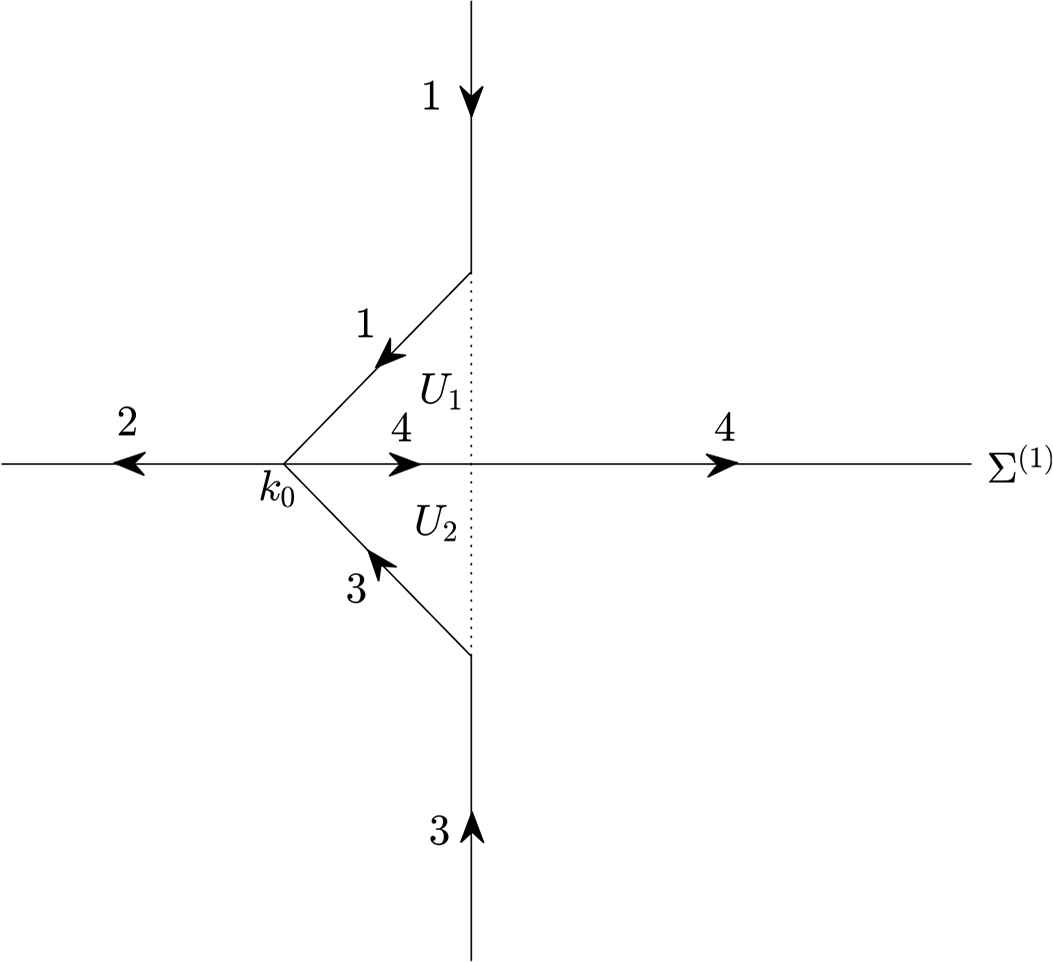
Then we obtain the RH problem
The jump matrix J(1)(x, t, k) is given by
Furthermore,
Remark 3.1.
It is noted that we introduce a 2×2 matrix-valued function δ(k) to remove the middle matrix term while we split the jump matrix
Since the jump matrix I + r†(k)r(k) is positive definite, the vanishing lemma [1] yields the existence and uniqueness of the function δ(k). By Plemelj formula, det δ(k) can be solved by
On the other hand, a direct calculation as in [17] shows that
Then we find that M(2)(x, t, k) satisfies the following RH problem
Before processing the next deformation, we will follow the idea of [3, 23, 24] and decompose each of the functions h, r1, r2 into an analytic part and a small remainder because the spectral functions have limited domains of analyticity. The analytic part of the jump matrix will be deformed, whereas the small remainder will be left on the original contour.
Lemma 3.1.
There exist a decomposition
- (i)
For each t > 0, ha(t, k) is defined and continuous for
- (ii)
For each ξ ∈ ℐ and each t > 0, the function ha(t, k) satisfies
for - (iii)
The L1, L2 and L∞ norms of the function hr(t,·) on iℝ+ are O(t−3/2) as t → ∞.
Proof.
Since h(k) ∈ C5(iℝ+), we find that
On the other hand, we have
Let
It is easy to verify that (3.28) imposes eight linearly independent conditions on the aj, hence the coefficients aj exist and are unique. Letting f = h − f0, it follows that
- (1)
f0(k) is a rational function of k ∈ ℂ with no poles in
- (2)
f0(k) coincides with h(k) to four order at 0 and to third order at ∞, more precisely,
The decomposition of h(k) can be derived as follows. The map k ↦ ψ = ψ(k) defined by ψ(k) = 4k2 is a bijection [0, i∞) ↦ (−∞, 0], so we may define a function F : ℝ → ℂ by
F(ψ) is C5 for ψ ≠ 0 and
By (3.29), F ∈ C2(ℝ) and F(n)(ψ) = O(|ψ|−1−n) as |ψ| → ∞ for n = 0, 1, 2. In particular,
Writing
Furthermore, we have
Hence, the L1, L2 and L∞ norms of fr on iℝ+ are O(t−3/2). Letting
We next introduce the open subsets The contour Σ(3) and the open sets 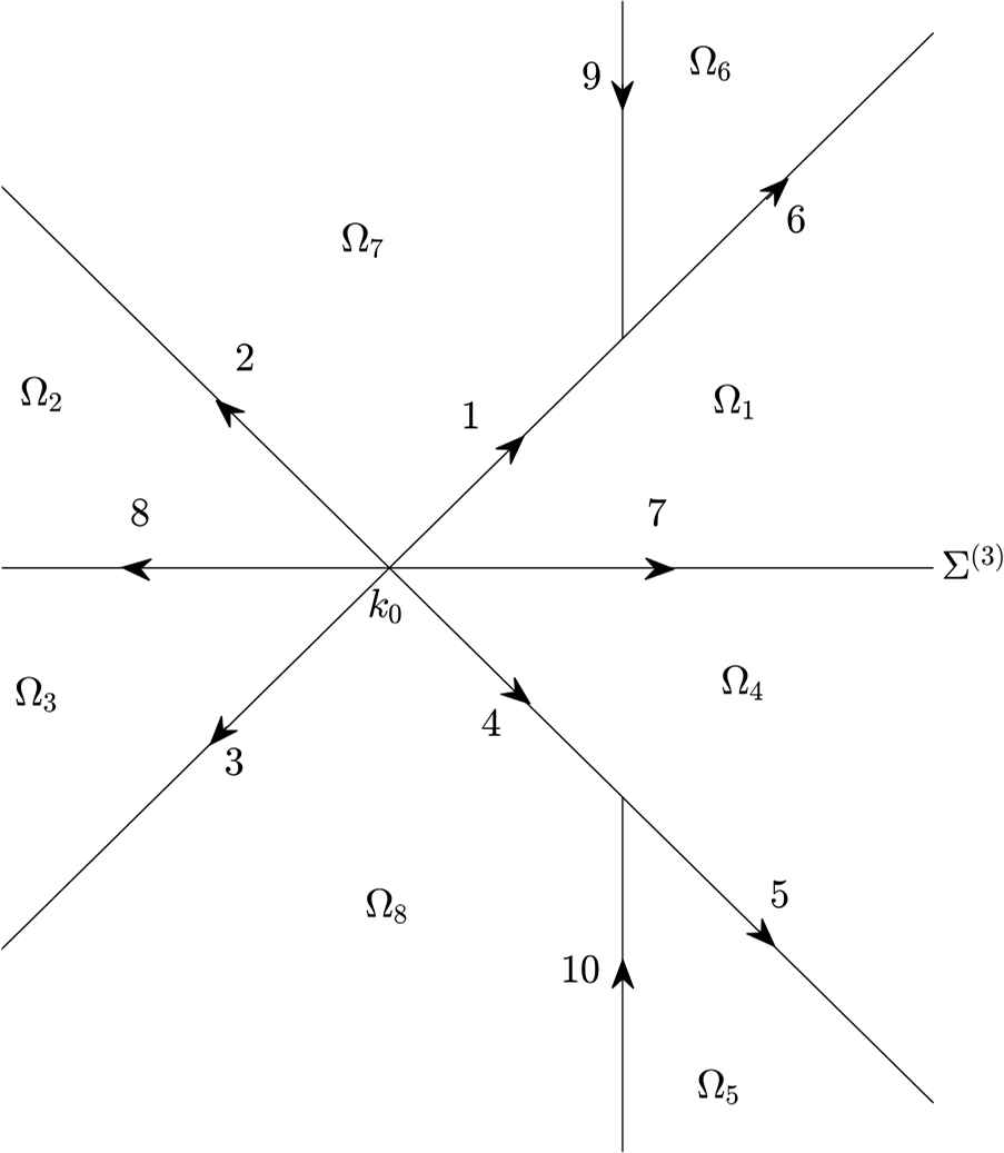
Lemma 3.2.
There exist decompositions
- (1)
For each ξ ∈ ℐ and each t > 0, rj, a(x, t, k) is defined and continuous for
- (2)
The functions r1,a and r2,a satisfy, for ξ ∈ ℐ, t > 0, j = 1, 2,
where the constant C is independent of ξ, k, t. - (3)
The L1, L2 and L∞ norms of the function r1,r(x, t, ·) on (k0, ∞) are O(t−3/2) as t → ∞ uniformly with respect to ξ ∈ ℐ.
- (4)
The L1, L2 and L∞ norms of the function r2,r(x,t, ·) on (−∞, k0) are O(t−3/2) as t → ∞ uniformly with respect to ξ ∈ ℐ.
Proof.
Analogous to the proof of Lemma 3.1. One can also see [17, 24].
The purpose of the next transformation is to deform the contour so that the jump matrix involves the exponential factor e−tΦ on the parts of the contour where ReΦ is positive and the factor etΦ on the parts where Re Φ is negative according to the signature table for Re Φ. More precisely, we put
Then the matrix M(3)(x, t, k) satisfies the following RH problem
Remark 3.2.
Recalling the meaningful work [3], begin performing the asymptotic analysis, the authors introduced a new spectral variable which led to a new phase function Φ(ζ, λ) = 4iλ2 +2iζλ only possed a single critical point, which has the same form as our phase function (3.6). Thus, it is not surprising that the figures of deformation contours similar to [3]. However, our jump matrices involved are all 3 × 3 (that is, the spectral functions r1(k), r2(k), h(k) are vectors) and the function δ(k) is a 2 × 2 matrix, which have the essential difference compared with [3]. As a result, the analysis in the next section will present some new skills, see Lemma 3.3.
3.2. Local model near k0
It is easy to check that the jump matrix J(3) decays to identity matrix I as t → ∞ everywhere except near k0. Thus, the main contribution to the long-time asymptotics should come from a neighborhood of the stationary phase point k0. To focus on k0, we make a scaling transformation by
Let Dε(k0) denote the open disk of radius ε centered at k0 for a small ε > 0. Then, the map k ↦ z is a bijection from Dε(k0) to the open disk of radius
For the first part in the right-hand side of (3.47), we have
Let
Lemma 3.3.
For
Proof.
The idea of the proof comes from [17]. It follows from (3.15) and (3.16) that
It follows from r2,a(r†r − rr†I) = r2,r(rr†I − r†r) that f(k) = O(t−3/2). Similar to Lemma 3.2, f(k) can be decomposed into two parts: fa(x, t, k) which has an analytic continuation to Ω2 and fr(x, t, k) which is a small remainder. In particular,
Then,
By the Cauchy’s theorem, we can evaluate I2 along the contour Lt instead of the interval (−∞,
Remark 3.3.
The estimate (3.50) also holds if r2,a is replaced with
Remark 3.4.
As mentioned above, here we use function detδ(k) which can be explicitly written down to approximate the unsolvable function δ(k) by error control. This procedure has never appeared in the long-time asymptotic analysis of the integrable nonlinear evolution equations associated with 2 × 2 matrix spectral problems.
In other words, we have the following important relation:
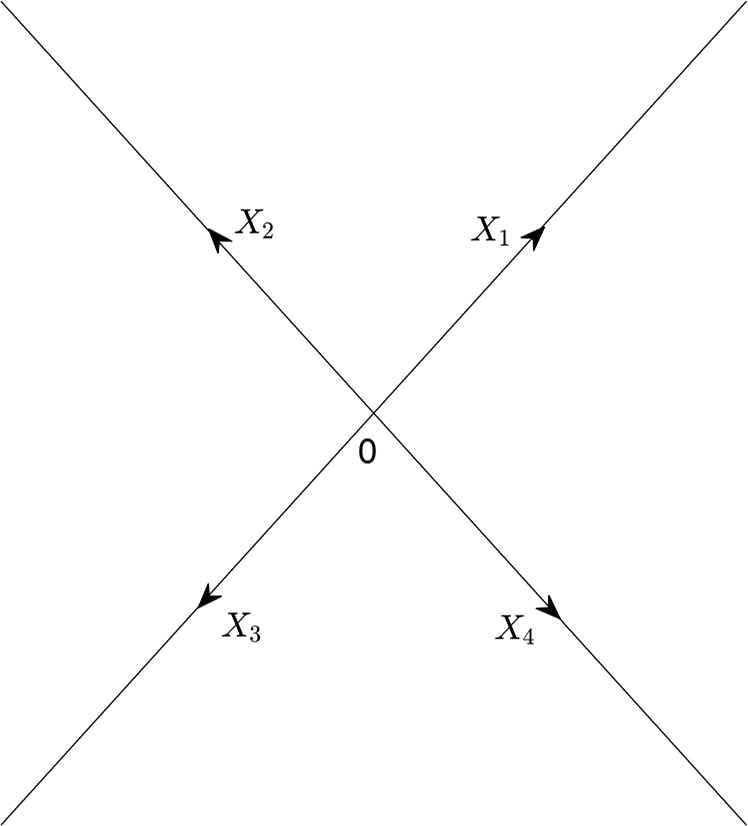
The contour X = X1 ∪ X2 ∪ X3 ∪ X4.
For any fixed z ∈ X and ξ ∈ ℐ, we have
Theorem 3.1.
The following RH problem:
Proof.
The proof relies on deriving an explicit formula for the solution MX in terms of parabolic cylinder functions. One can see [17].
Let Dε(k0) denote the open disk of radius ε centered at k0 for a small ε > 0 and 𝒳ε = 𝒳 ∩ Dε(k0). We can approximate M(3) in the neighborhood Dε(k0) of k0 by
Lemma 3.4
For each ξ ∈ ℐ and t > 0, the function M(k0)(x, t, k) defined in (3.64) is an analytic function of k ∈ Dε(k0) \ 𝒳ε. Furthermore,
Across 𝒳ε, M(k0) satisfied the jump condition
Proof.
The analyticity of M(k0) is obvious. Since |η| = 1, thus, the estimate (3.65) follows from the definition of M(k0) in (3.64) and the estimate (3.63).
On the other hand, we have
Then we have
By the general inequality
The norms on
If k ∈ ∂Dε(k0), the variable
Since
The estimate (3.67) immediately follows from (3.74) and
3.3. Derivation of the asymptotic formula
Define the approximate solution M(app)(x, t, k) by
Let
The contour
Let
Lemma 3.5.
For 1 ≤ p ≤ ∞, the following estimates hold for t > 3 and ξ ∈ ℐ,
Proof.
The inequality (3.79) is a consequence of (3.67) and (3.78). For k ∈ 𝒳ε, we find
Therefore, it follows from (3.65) and (3.66) that the estimate (3.80) holds. For
In a similar way, the estimates on
The results in Lemma 3.5 imply that:
This uniformly vanishing bound on Ŵ shows that the RH problem (3.77) is a small-norm RH problem, for which there is a well known existence and uniqueness theorem. In fact, we may write
The singular integral operator
It follows from (3.84) that
Using (3.80) and (3.86), we have
Similarly, by (3.81) and (3.86), the contribution from
By (3.82) and (3.86), the contribution from
Finally, by (3.68), (3.79) and (3.86), we can get
Thus, we obtain the following important relation
Taking into account that (3.7), (3.10), (3.13), (3.42), (3.76) and (3.89), for sufficient large
In view of (3.49) and (3.62), we obtain our main results stated as the Theorem 1.1.
References
Cite this article
TY  - JOUR
AU  - Boling Guo
AU  - Nan Liu
PY  - 2021
DA  - 2021/01/06
TI  - The Riemann–Hilbert problem to coupled nonlinear Schrödinger equation: Long-time dynamics on the half-line
JO  - Journal of Nonlinear Mathematical Physics
SP  - 483
EP  - 508
VL  - 26
IS  - 3
SN  - 1776-0852
UR  - https://doi.org/10.1080/14029251.2019.1613055
DO  - 10.1080/14029251.2019.1613055
ID  - Guo2021
ER  -