1. Introduction

In a previous paper [1], we displayed a time-independent Hamiltonian describing the motion of a charged particle moving in two dimensions under the combined influence of a magnetic field perpendicular to the plane of motion and a friction force proportional to the particle velocity. While, physically speaking, such a model arises via the coupling of the particle to a large number of external degrees of freedom, which are then averaged over, it was shown in [1] that it is possible to have a description via a time-independent Hamiltonian involving no additional degrees of freedom.

While time-dependent Hamiltonians for systems with damping are well-known, see for example [2], and arise in a fairly general way, time-independent simple Hamiltonians describing such systems are unusual. For a description of such Hamiltonians for the one-dimensional damped harmonic oscillator, however, see [3]. We presented—in the context of classical mechanics—the Hamiltonian model of the damped motion of a charged particle in a plane in the presence of a uniform magnetic field orthogonal to that plane in [1] and discussed its symmetry properties. Here we proceed to discuss the quantization of this model. For similar models involving the damped (one-dimensional) harmonic oscillator, the quantum behavior has been discussed extensively, see for example [4–6]. For two-dimensional models, such as the one we treat here, no such results are—to the best of our knowledge—extant.

The physical relevance of such a quantum treatment may at first sight appear questionable: indeed, damping generally arises from interaction with other degrees of freedom, which are then averaged over, and such a procedure, in quantum mechanics, leads to a non-unitary time evolution, in which pure states evolve into mixtures. Nevertheless, it may be of some interest, from a mathematical viewpoint, to understand how a Hamiltonian system which mimics exactly a damped system, behaves when appropriately quantized. We shall later argue, however, that some of our results do indeed confirm the doubts concerning the physical appropriateness of such a quantization procedure.

Several interesting questions arise. In particular, since motion in a damped system eventually stops, the system eventually reaches a state in which both its position and its velocity are fixed. The way in which this is reconciled with the Heisenberg uncertainty relation is that, since the Hamiltonian is not of the usual form, the connection between momentum and velocity is not the usual one. But it is the momentum which is conjugate to position, and which thus must thus satisfy the uncertainty relation. Since in the limit of velocity tending to zero, the connection between velocity and momentum is seen to become singular, one finds that the contradiction to the Heisenberg uncertainty relation is indeed avoided.

Below, we shall look at the propagator of the Hamiltonian. Physically, this tells us how a state evolves in time. We shall discuss three representations of this propagator: in Section 3 we shall compute it in momentum space and we shall further show that the spectrum of the Hamiltonian is continuous and infinitely degenerate. From this follows that the evaluation of eigenfunctions has little interest, since there is no obvious way to determine a physically reasonable choice of eigenfunctions among the infinitely many possibilities. Since momentum does not have a clear physical significance, however, we turn in Section 4 to the evaluation of the propagator in position space. It can indeed be evaluated explicitly. Nevertheless, this expression also does not readily reflect the correspondence between what happens at the quantum and the classical levels. In Section 5 we give yet another expression for the propagator in terms of variables corresponding to the actual velocity, as opposed to the momentum, and obtain an expression, in which the connection to the classical motion becomes readily apparent.

2. The model

The model is given by the following Hamiltonian:

Here E, P, a and b are 4 a priori arbitrary (real) parameters; the two canonical variables x respectively y are the two Cartesian coordinates of the (charged) particle moving in the plane and p_x respectively p_y the corresponding canonical momenta.

This Hamiltonian features the following conservation law, as described in [1]:

It yields the following equations of motion:

which can be rewritten equivalently in terms of the velocities alone: let be the modulus and the phase of the classical velocity vector. The equations of motion then read:

Note the the parameters P and E do not enter in these equations of motion (2.2). We shall nevertheless maintain them, both on dimensional grounds, and as they play a role in the quantized version of the system.

Note that a further classically irrelevant parameter θ can also be readily introduced: indeed, the Hamiltonian (2.1a) is not invariant under rotations of the positions and the momenta by the same angle. If we perform this operation, we obtain the more general Hamiltonian:

which again generates the equations of motion (2.2), since these are invariant under rotations of the positions. Due to its complexity, we shall not analyze this Hamiltonian (2.3) and shall always limit ourselves to Hamiltonian (2.1a). The final results for the Hamiltonian corresponding to θ = 0 can, however, easily be extended to the general case by performing the appropriate rotation in the position and momentum variables. For further remarks on the classical Hamiltonian, see [1].

3. The quantum-mechanical propagator in the momentum representation

Quantizing the Hamiltonian (2.1a) is not straightforward in position space. Indeed, in that context, the momenta p_x ⇒ −i∂/∂x and p_y ⇒ −i∂/∂y are differential operators, so that the operators exp(p_x) and cos(p_y) are differential operators of infinite order. In fact, as it turns out, the latter is a combination of translations by 1 and −1, whereas the former, defined only on entire functions, is a translation by −i. Note that we assume throughout that dimensions are set so that ħ = 1.

On the other hand, if one quantizes in the momentum picture, everything is quite straightforward. The quantization procedure is given by

If we now consider the time dependence of the state ψ in the momentum representation, which we take to be represented by the function ψ^(px,py;t), the time-dependent Schrödinger equation assumes the form

This is a linear PDE of first order, and therefore solvable using the method of characteristics. Defining ψ^0(px,py) as the initial value ψ^(px,py;0), the result is given by

This explicit form of the propagator can be connected to the classical equations of motion for the momentum. Indeed, at the classical level, we have

But from (3.3) follows

The classical behaviour is thus reflected exactly in the quantum behaviour as far as the probability distribution for the momenta is concerned. However, this does not really give a great deal of information, as the momentum does not have an obvious physical significance. Moreover, the probability distribution of the momenta is quite insufficient to reconstruct the state ψ. We should therefore attempt to obtain a representation for the propagator which is more closely connected to the classical behaviour. We show in the next Section how to evaluate the same propagator in the position representation.

4. The propagator in position space

We first transform the function ψ^(px,py;t) to the position representation:

where K(ξ, η) is defined as

This can be evaluated explicitly as follows. First we note that the integrand is 2π-periodic in p_y. Let g(p_y) be an arbitrary such function. One then has

Hence, we now define

Let us therefore start by evaluating the following integral

We can rewrite the term in the exponential as

where (here and hereafter; see (3.3)) and ϕ(t) is a phase which depends in some way on the time t, but which, as we shall see, does not enter in any way in the final answer.

We may now express the integral S_n(p_x) as

where J_n(z) is the Bessel function of order n [7]. We obtain in this manner

Shifting p_x by −ln[A(t)/ρ] yields

where the final transformation is obtained by setting w = exp(p_x/P). The final integral is a Mellin transform of J_n(w), which can be found using Mathematica or in tables, so that one finally obtains

By substituting (4.11) into (4.4) the final result is obtained. The final expression for the propagator thus reads

Again, however, the result is not easy to interpret physically. In particular, it is initially surprising that the propagator is concentrated on integer values of η, in other words, that, from any value of y, the system can only move to another value y′ satisfying y′ − y ∈ 𝕑, whereas no corresponding restriction holds for x.

As was pointed out in [1], the Hamiltonian (2.1a) is not rotationally invariant, even though its classical orbits have the property that rotating one orbit leads to another such orbit. In other words, rotations yield a symmetry of the equations of the motion, but not of the underlying Hamiltonian structure. This can be restated by remarking that the Hamiltonians defined by (2.3) are inequivalent for different values of θ. This is quite clear in this case, since upon performing a rotation of the x and y variables by an angle θ, the y axis is rotated into an arbitrary position, and it is along this new axis that the propagation occurs via discrete jumps. The Hamiltonians (2.3) for different θ thus have quite different quantizations. Similarly, as can readily be observed, the classically irrelevant quantities E and P play an important role in the quantum propagator, even in the position representation.

This hints at a serious difficulty in this proposal of a “quantization” of a system involving damping: different Hamiltonians leading to the same equations have altogether different quantizations, even in the position representation.

It appears likely that a semiclassical computation, involving transitions for large values of both ξ and η, would lead back to the classical behavior, and thus to equivalent behaviors for all versions of the Hamiltonian. This is a rather forbidding computation, however, which we have not undertaken. Rather, we identify yet another representation, more in line with a group-theoretic structure underlying the system (2.1a), in which the connection to the classical dynamics is made more explicit.

5. The propagator in “natural” variables

Define the operators

These satisfy, together with the operators x and y, the commutation relations:

with all the other commutators between the four operators x, y, v_x and v_y vanishing. These thus form a Lie algebra, so that the exponential of any linear combination of them belongs to a group G which, as we shall see, is isomorphic to the two-dimensional Euclidean group.

Since the Hamiltonian (2.1a) is such a linear combination, it follows that the propagator as a function of t is a one-parameter subgroup of G. In the following, we aim to find a representation for the time evolution of the Hamiltonian (2.1a) which takes this fact into account.

Note that the 4 objects defined in (5.1) are operators: in other words, they operate on the abstract state ψ in different ways according to the representation in which ψ is given. Thus, in the momentum representation, we have

And equivalently, in the position representation, we have

Note that, if we use these operators, the Hamiltonian (2.1a) reads

and that the commutation relations (5.2) imply that

This justifies therefore the nomenclature introduced above: v_x and v_y are proportional to the velocities in the usual sense, whereas the momenta have no simple significance in terms of the velocities.

We now start to define a function ψ˜(vx,vy) which expresses the quantum mechanical state in terms of the observables v_x and v_y. To this end, we first observe the need for care, since the transformation connecting (p_x, p_y) with (v_x, v_y) is not one-to-one. Indeed, to every vector (v_x, v_y) there corresponds only one value of p_x, but an infinite set of values of p_y given by −Parctan(v_y/v_x) + 2πnP for all integer values of n. We thus define for every Q

Here v_x and v_y are connected to p_x and p_y via (5.1). Note that the Jacobian of the transformation from v_x and v_y to p_x and p_y reads as follows:

We shall thus always incorporate the factor (E/P)2exp(2px)=(vx2+vy2)/P2 in any “scalar product” integration related to the change of variables from p_x, p_y to v_x, v_y, without changing the normalization of the corresponding wave functions.

Let us now discuss the meaning of the parameter Q (see (5.7)): since v_x and v_y are invariant under discrete translations of p_y by 2πP, we may classify their eigenstates according to the eigenvalue under the effect of that discrete translation. This is altogether similar to the Bloch vector in the theory of periodic potentials, except that, since we are dealing with translations in p_y, the corresponding eigenvalue could be called a “Bloch position” which is why we named it Q. As is readily seen, both v_x and v_y and the position operators x and y leave Q invariant, so that we may without difficulty limit the study of the time evolution of our system to a sector of constant Q, since this remains constant over time. By its definition Q can clearly be limited to the values between 0 and 1/P.

Let us now express ψ˜(vx,vy;Q) in terms of the original function ψ(x, y). From (5.7) follows

where here the arctangent only runs from −π to π. Using Poisson’s summation formula, see [8], we obtain

If we now go over to a description in polar coordinates, by setting

where v=vx2+vy2 is the modulus and ϕ = arctan(v_y/v_x) the phase of the 2-vector (v_x, v_y), so that we have

Several features of this expression are deserving of comment: first, the expression is not 2π-periodic in ϕ, but it only fails to be so due to the factor exp(−iPQϕ), due to the “Bloch position” Q. Second, the function Ψ˜(v,φ;Q) viewed as a function of the phase ϕ of the velocity is the discrete Fourier transform of the function ψ(x, y) where y is taken over all integer multiples of 1/P shifted by Q. Finally, the function Ψ˜(v,φ;Q) of the modulus v and the function ψ(x, y) as a function of x are related by a Fourier transform evaluated at lnv.

Note that, as stated above, the scalar product between two functions of the two variables v_x and v_y is computed using the surface element dv_xdv_y defined in (5.8). Rewriting this in polar coordinates (see (5.12b)), we obtain

This means we shall always compute scalar products between two functions in the variables v and ϕ using the surface element (5.14), which implies that, for example, an operator such as iv∂_v is self-adjoint.

By definition (see (5.12b)) it is clear that v_x and v_y act on Ψ˜(v,φ;Q) as multiplication by vcosϕ and vsinϕ respectively. We now describe the actions of the operators x and y in this picture. Clearly one has

The operator x thus acts on ψ˜(vx,vy;Q) as the operator iP⁻¹v∂_v. Note that this operator is indeed self-adjoint when the scalar product is defined over the volume element dvdϕ/v.

Similarly we have

hence the operator −iP⁻¹∂_ϕ multiplies the function ψ(x, m/P − Q) by m/P − Q, and thus has the same effect as the operator y acting on ψ(x, y).

The time-dependent Schrödinger equation satisfied by the function Ψ˜(v,φ;Q) therefore reads

Here we see that the behaviour of the characteristics of the equation matches exactly the classical behaviour. Indeed, the characteristic equations are

They are the time-reversed version of the Newtonian equations of motion (2.2c). The peculiar quantum feature is now the variation in phase induced by the first term of the equation. It thus follows that any wavepacket that is well localized in the variables v and ϕ would have a quantum development that is well determined by, and analogous to, the classical motion.

Let us consider as a specific instance an initial condition in the form of a coherent wavepacket ψ₀(x, y) ≡ ψ(x, y;0) defined in the standard “shifted Gaussian” way:

Here x¯ and y¯ denote the average positions in the x and y directions, and p¯x and p¯y the corresponding average momenta.

Since ψ₀(x, y) factorizes into an x and a y dependent part, the corresponding Ψ˜0(v,φ;Q) factors into a radial part V(v; Q) and an angular part Φ(ϕ; Q):

We find, using Mathematica:

Here θ₃(z, q) is a theta function, as defined in [7]. It is readily seen that localization in the physical variables v and ϕ, in the sense that the variance of these quantities are much less than their average values, arises whenever the dimensionless parameters ω/px,02 and ω/P² are much smaller than 1. This is illustrated in Figure 1. In the spirit of the Heisenberg uncertainty relation, this corresponds to a rather large uncertainty in the position representation. However, if we choose the average values x₀ and y₀ sufficiently large, we still have a small relative uncertainty. For such initial conditions, therefore, a time evolution close to the classical one is recovered.

Fig. 1.

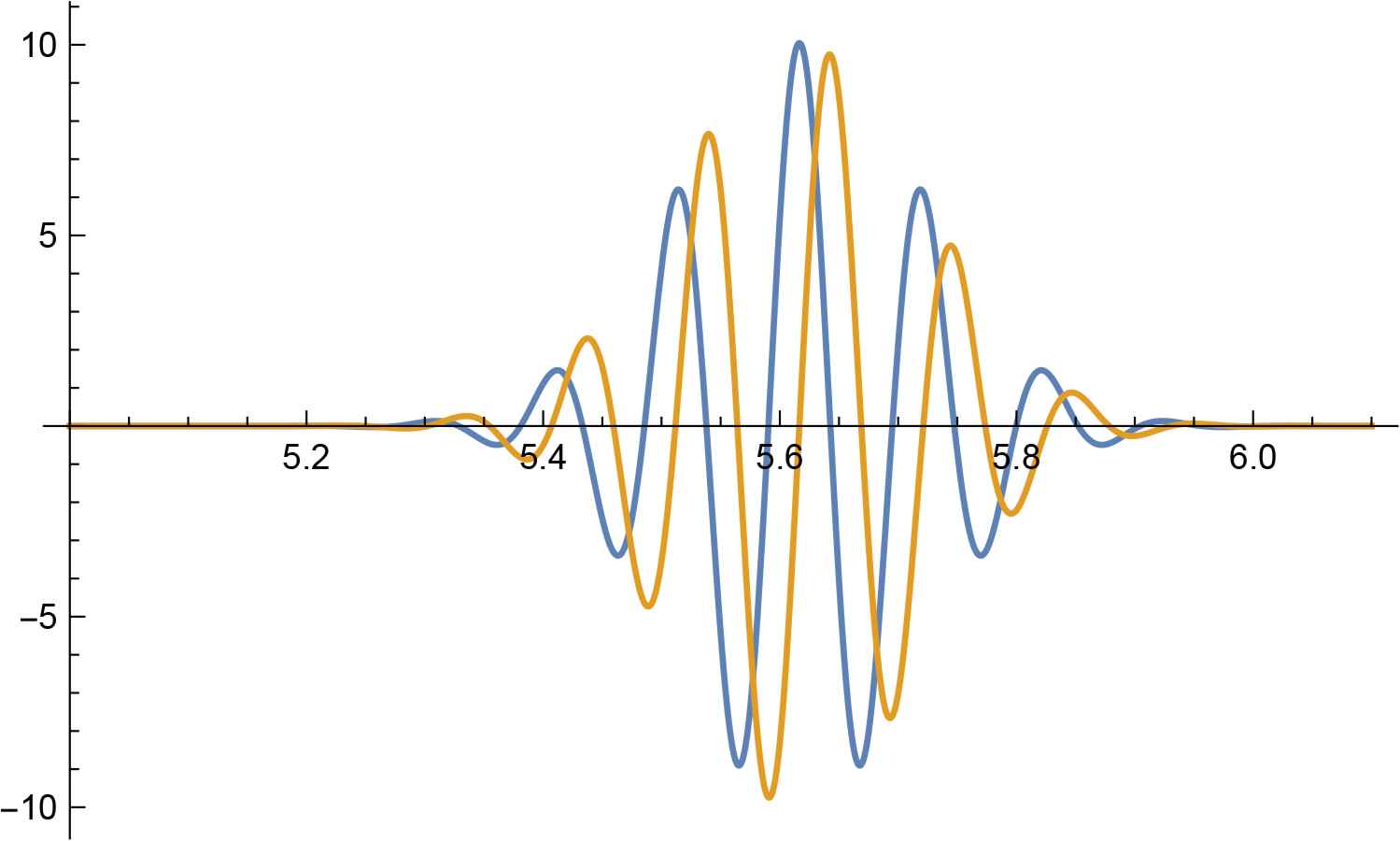
Plot of the real (blue) and imaginary (yellow) part of Φ(ϕ) for the following values of the parameters: Q = 0, P = 3, ω = 0.1, y¯=20 and p¯y=2. Outside the plotted interval, the function is altogether negligible. The function is 2π-periodic. Note both the already fairly high degree of localization and the similarity to an ordinary coherent state.

As a consistency check, we note that, if ω/P² ≪ 1, the sums arising in (5.13) are Riemann sums where P determines the integration step. They are thus to a good approximation independent of the value of P. as is indeed to be expected for a time evolution close to the classical one.

Profoundly non-classical is the conservation of Q, which is an integral of motion having no analog in classical dynamics. One could attempt to make wavepackets that are yet more classical than the ones here considered by taking superpositions of a continuum of different values of Q. However, while the wave functions defined by (5.13) are indeed not periodic, due to the term exp(iPQϕ), they remain nearly periodic, in the sense of being like Bloch waves. Were we to combine different values of Q, this simple behaviour would altogether disappear and the interpretation of ϕ as the angle of the velocity vector would not be sustainable any more. It is, in any case, satisfactory that, in the semiclassical limit, which involves ωy02≫1 and ω/P² ≪ 1, we naturally have y₀P ≪ 1, and hence, since PQ < 1, we have y₀ ≫ Q. This being the case, we see that the influence of the essentially quantum symmetry Q is negligible in the semiclassical limit.

6. Conclusion

To summarize, we have introduced a Hamiltonian (2.1a) which describes classically the dynamics of a particle that moves in a plane in the presence of a constant magnetic field perpendicular to that plane, and is additionally subject to a friction force linearly proportional to the velocity. This corresponds to the equations of motion (2.2a), which are indeed the Hamiltonian equations for (2.1a). The Hamiltonian H_R defined by (2.1a) depends on 4 parameters, namely a, b, E and P, of which only the first two appear in the classical equations of motion, a being the damping coefficient and b the magnetic field. The Hamiltonian can be further changed without modifying the classical equations of motion, in particular, the family (2.3) also gives the same equations of motion for the positions of the particles.

This follows immediately from the fact that H_R(p_x, p_y; x, y|θ), see (2.3), arises from the Hamiltonian defined in (2.1a) by a rotation of the coordinates, which clearly transforms an orbit of (2.2c) into another such orbit.

In the quantum version of the system, we evaluate the time evolution of the system, and find that both in the momentum representation and the position representation, the parameters E and P play an important role. Additionally, one sees that, in the propagator in the position representation, the motion in the y direction has a completely different nature than in the x direction, since, in the y direction, only integer changes in the value of y can occur, whereas no such restriction exists for x. Clearly, this means that the various Hamiltonians defined in (2.3) all have different behaviors in the quantum regime. Since there is no reason to prefer any particular value of the parameters E, P and θ, as all describe the classical dissipative behaviour equally well, we find that the quantization procedure is highly nonunique.

On the other hand, we have found a representation in the “velocity” variables in which the equations take a very similar form to the classical equations. In that case it is indeed possible to identify initial conditions, analogous to coherent states, which behave approximately classically, and for these cases we do indeed find that the parameters E and P are approximately irrelevant, and also that the evolution is isotropic in x and y, so that θ also does not matter.

Acknowledgments

Financial support from the grants CONACyT 254515 and DGAPA–PAPIIT–UNAM IN103017 is gratefully acknowledged, as well as the hospitality of the Centro Internacional de Ciencias in Cuernavaca and of the Dipartimento di Física of the Università degli Studi “La Sapienza” in Rome, where part of this research was carried out.