
Analytical Cartesian solutions of the multi-component Camassa-Holm equations
- DOI
- 10.1080/14029251.2019.1591725How to use a DOI?
- Keywords
- Solution; Analytical Cartesian solution; Camassa-Holm equation; Curve integration theory; Multi-component Camassa-Holm equations
- Abstract
Here, we give the existence of analytical Cartesian solutions of the multi-component Camassa-Holm (MCCH) equations. Such solutions can be explicitly expressed, in which the velocity function is given by u = b(t) + A(t)x and no extra constraint on the dimension N is required. The advantage of our method is that we turn the process of analytically solving MCCH equations into algebraically constructing the suitable matrix A(t). As the applications, we obtain some interesting results: 1) If u is a linear transformation on x ∈ ℝN, then p takes a quadratic form of x. 2) If A = f(t)I + D with DT = −D, we obtain the spiral solutions. When N = 2, the solution can be used to describe “breather-type” oscillating motions of upper free surfaces. 3) If
- Copyright
- © 2019 The Authors. Published by Atlantis and Taylor & Francis
- Open Access
- This is an open access article distributed under the CC BY-NC 4.0 license (http://creativecommons.org/licenses/by-nc/4.0/).
1. Introduction
Exact solutions of mathematical physics are usually very important. Not only because they can help us to understand physical phenomena they describe in nature, but also because they can serve as benchmarks for checking and improving numerical codes developed for studying more complex problems. Therefore, a lot of powerful methods has been developed, such as inverse scattering method, Hirota direct method, Darboux transformation and Bäcklund transformation et al [1–10]. However, none of these methods is universal due to the diversity and complexity of PDEs. Therefore, it will be of interest to find other effective methods that can lead to exact solutions.
In this paper, we shall adopt a new method to construct solutions of the multi-component Camassa-Holm-type (CH) equations, which takes the following form [11]:
To motivate our study, we shall review some related progresses on the multi-component CH system. The original interest in it may go back to the Camassa-Holm equation
We notice that most existing papers deal with the case n = 1 or 2. Investigations on the multi-component CH system mentioned above are rare, expect for the work done in [11, 34, 40, 41]. In particular, little work has been done on seeking exact solutions. From the view of mathematics and physics as explained in [40, 42, 43], the multi-component CH system is also very interesting. This deeply motivates us to undertake the present investigations.
Here, we would like to seek exact solutions with the velocity field of the form
The structure of the paper is as follows: In section 2, we show that the multi-component CH equations admit the analytical Cartesian solutions if A satisfies certain matrix differential equations. In section 3, two solvable reductions are considered. Firstly, if A is an antisymmetric constant matrix, then the multi-component CH equations admit exact Cartesian solutions. Secondly, to construct more general solutions, the technique of matrix decomposition is used to make the matrix ODEs solvable. In particular, when N = 2, we obtain the rotational spiral solution and irrotational elliptical solutions obtained by Zhang, An and Yuen et al. The former can be used to describe the motion of “breather”-type oscillations of free surfaces in the upper ocean and the latter can be used to describe the drifting phenomena. In section 4, we discuss the property of such Cartesian solutions. Finally, a short conclusion is attached.
2. Existence of the exact Cartesian solutions
For convenience, we introduce a transformation via
Here, our main goal is to seek suitable function p that enables us to obtain the analytical solutions wherein the velocity function u takes a linear form
It is noticed that ρ is redefined by p via (2.1), therefore, we only need to deal with p for solving the multi-component CH equations (2.2).
Theorem 2.1.
Defining B as part of a matrix Riccati equation
If A and B satisfy the following matrix differential equations
In the above, b(t) is a vector function and c(t) is a scalar function c(t), which satisfy the following matrix ODE equations:
Proof.
We now first prove the proposed analytical solution (2.6) will lead to (2.7) by solving the equation (2.2)1. Substitution (2.6) into the first equation of (2.2) yields
For the convenience of subsequent computations, an auxiliary matrix is introduced via
It is noticed that for solving p(x, t) from the above equation, all the N equations must be compatible with each other. In other words, the vector functions (Q1, Q2,...,QN) should be a potential field of p wherein the sufficient and necessary conditions are
The above condition implies that
The condition (2.18) shows that the function p(x, t) can be written into a complete differential form
Therefore, we obtain that the second kind of curvilinear integral of p(x, t) is independent of path. So that it allows us to take a special integration route from (0, 0,...,0) to (x1, x2,...,xN)
Directly complicated calculation shows that
At this point, we have finished proving that the functions given by (2.6) and (2.7) satisfy the first equation of (2.2). In the sequel, we shall prove that such functions also satisfy the second equation of (2.2). On use of the relations (2.5), (2.8) and (2.9), we have
Hence we obtain the following relation
To conclude, here we have theoretically obtained the existence of explicit Cartesian vector solutions of (2.2) in Theorem 2.1. The Cartesian solutions are mainly governed by A via the relation (2.5), which is a complex matrix ODE system involving N2 scalar equations. As we know, compared with a scalar equation, it is usually very difficult to construct general solutions of a given matrix ODE system. Therefore, to make some solutions available, special techniques are devised in the subsequent section.
3. Special reductions and corresponding solutions
Now, we return back to the condition (2.5) given in Theorem 2.1. Due to the inherent complexity to solve matrix ODE, our attentions are restricted to the cases that lead to some special solutions.
I. The first reduction: A is an antisymmetric constant matrix
It is noted that when A is an antisymmetric constant matrix, the solution can be readily constructed, which is established in the following theorem:
Theorem 3.1.
If A is an anti-symmetric constant matrix, then the multi-component CH equation (2.2) admits a general solution via
Proof.
Since the solution derived here is just a special case of Theorem 2.1. we just need to validate that the conditions (2.4), (2.5), (2.8) and (2.9) can be satisfied in Theorem 3.1.
When A is an antisymmetric constant matrix, the conditions (2.4) and (2.5) can be easily checked. Insertion of A into (2.8) and (2.9) delivers
Computation shows the solutions of them are just (3.3) and (3.4).
As the application of Theorem 3.1. here we give an illustrative example:
Example 3.1.
Taking N = 2, for the 2-dimensional multi-component CH equations, setting the anti-symmetric matrix A as
To shed lights on the behaviors that the solution derived may exhibit, we perform the numerical simulations in Fig. 1. There we choose c1 = c2 = 1, c3 = c4 = 0. From the figure, we can see that the steady flow is rotational and the velocities of all fluid particles point directly inwards to the origin, which are quite different from those in the radially symmetric solution case.
The structure of the 2-dimensional rotational solution with velocity u = (u1, u2)T given in (3.6). The length of the arrow stands for the strength of the velocity field.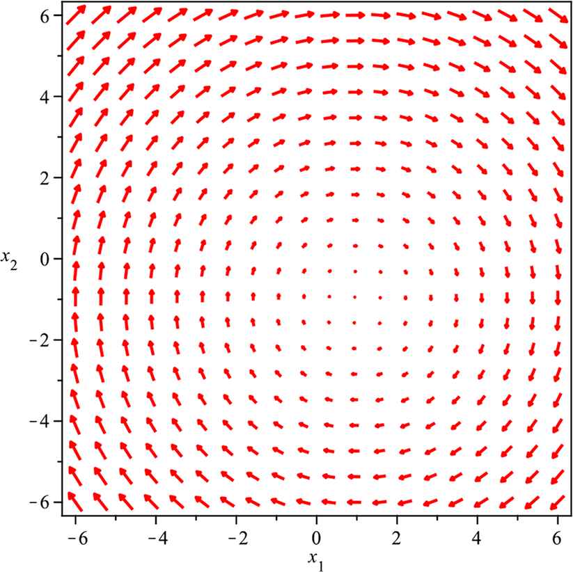
Example 3.2.
Taking N = 3, for the 3-dimensional multi-component CH equations, setting the anti-symmetric matrix A as
So according to (3.1) and (3.2) we can get the following rotational solution:
II. The second type reduction: A is a decomposable t-dependent matrix
The special case considered here is A being a certain decomposable time-dependent matrix. In particular, we discuss the two cases: one is A = f(t)I + D with D antisymmetric and the other is
Theorem 3.2.
Suppose that the matrix A can be decomposed into
Proof.
With the aid of (3.8) and (3.9), one can have
In the sequel, we shall show the condition (2.5) can be also satisfied under conditions given in this theorem. On using (3.12) and (3.8), we can obtain
The proof is completed.
In the following, we shall mainly focus on two special cases. One case is when E = f(t)I, D ≠ 0 to be discussed in Corollary 3.1. The other case is when
Corollary 3.1.
In Theorem 3.2, setting
Proof.
On inserting (3.13) into (3.9), one can have
Hence, the solution of D is derived in (3.14). While substituting (3.13) into (3.7), one can directly obtain (3.16) and the condition (3.11) is satisfied automatically.
It is noticed that the equation (3.16) can be rewritten into a form of
Thus, in what follows, we shall show its solvability in two cases:
-
Case 1. If ft + (N + 1) f2 = 0, then the system (3.18) has a solution
where k1 is a constant of integration. Then insertion it into (3.14) giveswith C is an antisymmetric matrix of integration whose elements satisfy (3.15). -
Case 2. If ft + (N + 1) f2 ≠ 0, on introduction a function g via
whereIntegration (3.22) with respect to t shows that
which can be readily written intoTherefore, we can obtain the following relation
In the above, k2 is an integration constant. Here we go with k2 ≠ 0. By multiplying
Its solutions can be readily obtained by trigonometric substitutions, whose forms are dependent on the parameters k2 and k3. Here we just take k2 > 0 and k3 > 0 as the example to illustrate. Under this condition, we introduce the trigonometric substitution of this form
Once N is given, the value of (3.27) can be known. So that g and f can be generated accordingly via (3.21). Once f is generated, the function of D will be obtained via (3.14). Therefore the analytical solutions under Case 2 is derived.
Remark 3.1.
For other choices of k2 and k3, one needs to introduce the corresponding trigonometric substitution to find the iterative relation similar to (3.27). Here the calculations procedures are omitted.
Remark 3.2.
We needs to point out that when k2 = 0, from (3.23), we can obtain that g is governed by
Insertion it into (3.21) shows that
If we choose h1 = 1 and h2 = k1, it is nothing but the solution given in (3.19) in Case 1. Thus, we conclude that the solutions (3.27) obtained in Case 2 are more general.
As the application of the above corollary, we give some examples:
Example 3.3.
Taking N = 2, according to Case 1, we choose k1 = 0, b(t) = 0, c(t) = 0 and A as
Therefore, we can obtain an exact solution
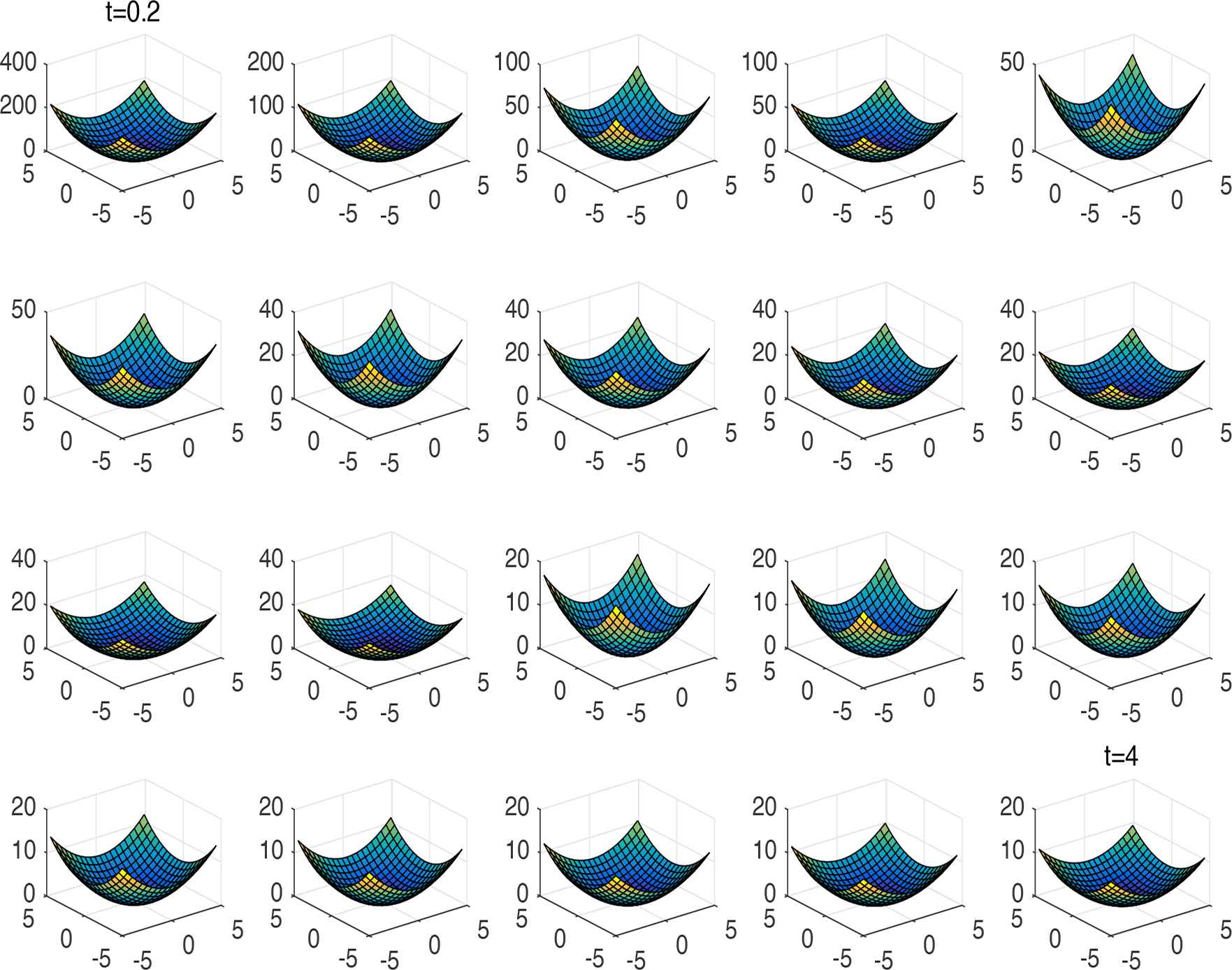
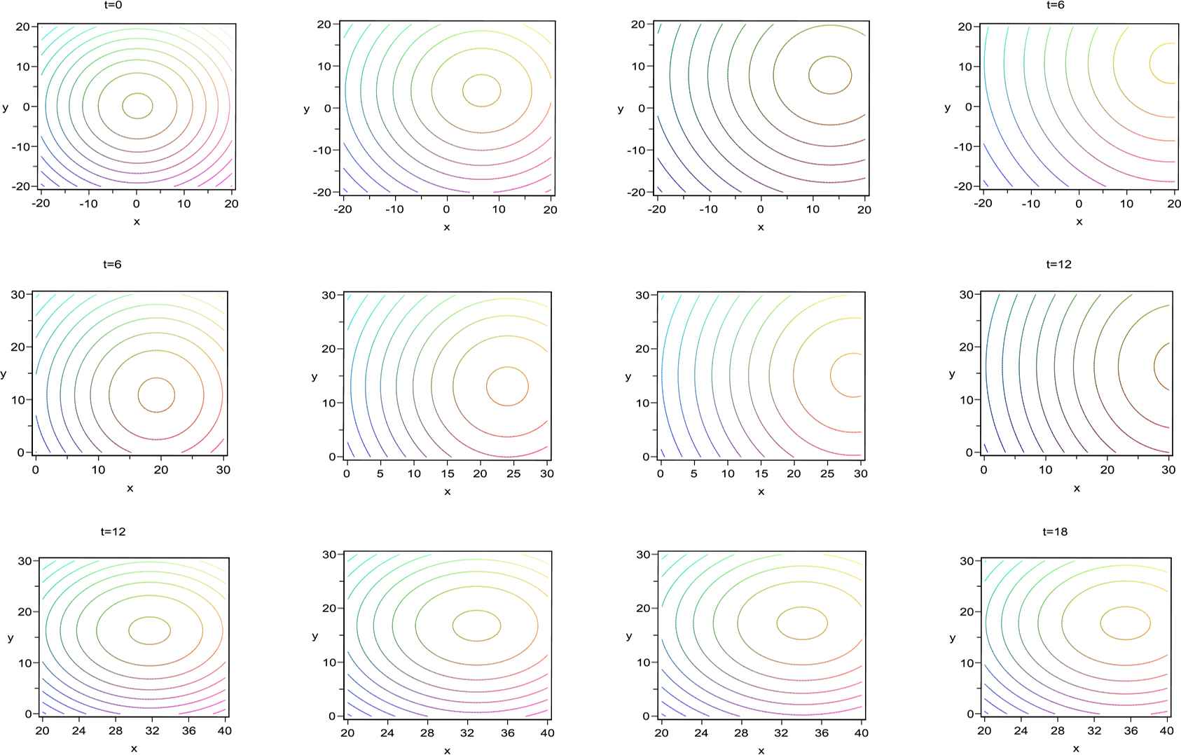
It is a kind of spiral solution that presented by Zhang and Zheng for Euler equations [52]. Interestingly, here we obtain for the multi-component CH equation. The behaviors of the spiral solution is exhibited in Fig. 2 and Fig. 3. We find from Fig. 2 that the velocities of all fluid particles point directly from the origin to the outside, which are quite different from the rotational solution obtained in (3.6). From Fig. 3, we find the surfaces of p jump up and down with time changing. It is remarkable that such jumping up and down phenomena just coincide with the motion of the “breather-type” oscillations of upper free surfaces in the ocean.
The structure of the 2-dimensional spiral solution with u = (u1, u2)T given in (3.30). The length of the arrow stands for the strength of the velocity field. Time evolutions of the solution 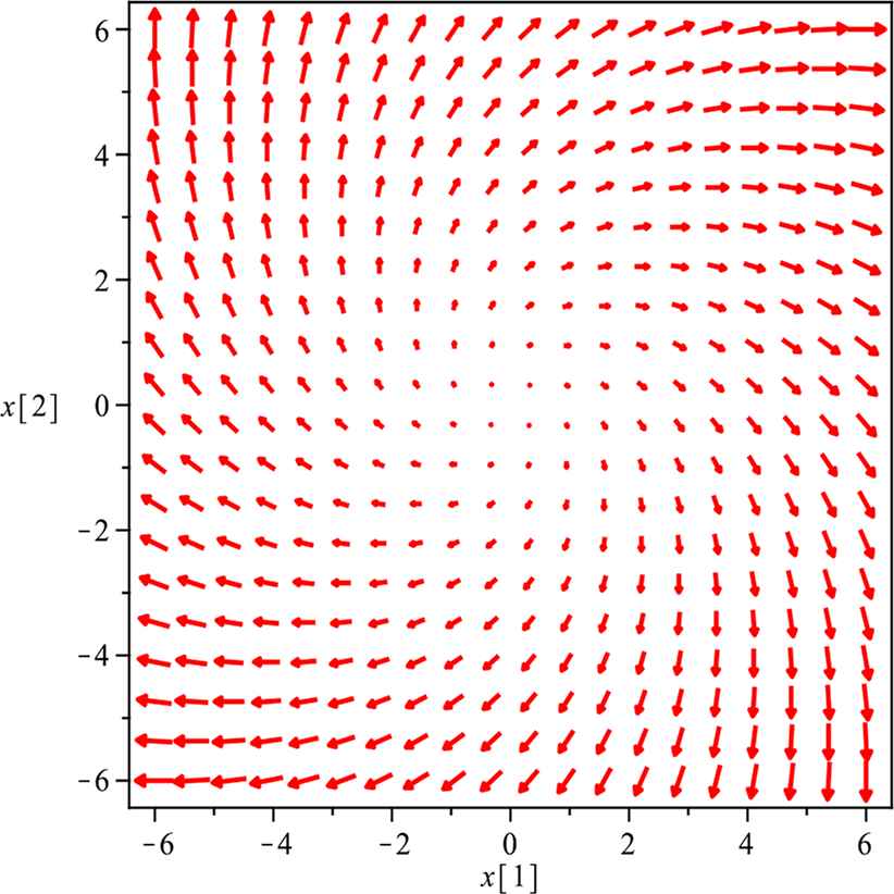
Corollary 3.2.
In Theorem 3.2, if setting
Then it is obvious that the relations (2.9)–(2.11) in Theorem 3.2are satisfied. Meanwhile,
Example 3.4.
Taking N = 1, for 1-dimensional CH equation, we choose c(t) = 0 and
Therefore, we obtain an analytical solution
In particular, if we choose b(t) = 0 and c(t) = 0, this solution is just what has obtained by Yuen [53].
Example 3.5.
If N > 1, we choose
So that we obtain the general analytical solution
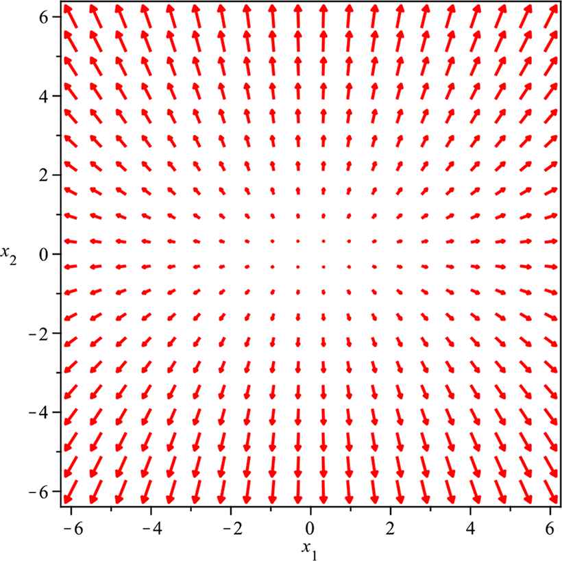
The structure of the 2-dimensional irrotational solution with u = (u1, u2)T given in (3.36). The length of the arrow stands for the strength of the velocity field.
Time evolutions of the solution p given in (3.36). Here C1 = 5, C2 = 3, α = 1, μ = −1, β = 0 and the time interval Δ = 3.
4. Quasi-linear superposition principle of solutions
In order to shed some light on the properties and structures of the solutions, we now return back to the solutions (2.6) and (2.7). We take b(t) = 0 and c(t) = 0 for simplicity so that the solutions is reducible to
This renders one to consider that the solution u(x) is generated by a linear transformation A on x ∈ ℝN:
It is noticed that there exists a quasi-linear superposition principle for Cartesian solution (4.1) that is analogous to the linear equations:
Theorem 4.1.
Suppose that A and B satisfy the conditions in Theorem 2.1, and u(x), u(y) are two solutions whose take the form of (4.1). Then
5. Conclusions and discussions
The multi-component CH system is an important mathematical physics model, which has been wide used in fluid mechanics, geophysics, oceanic dynamics and nonlinear optics et al. In the paper, based on the matrix theory and curve integration theory, we have shown that the multi-component CH equations admit analytical Cartesian solutions. Such solutions globally exist and admit a quasi-linear superposition principle under the condition b(t) = 0 and c(t) = 0. As applications, we give some interesting solutions and their numerical simulations. Among these solutions, some are more general than other researchers obtained before. While, to our knowledge, some are completely new. However, there are still some interesting problems that need further consideration:
- 1)
It is seen that seeking the suitable matrix solution A in (2.5) proves key to derivation of analytical solutions of the multi-component CH equations. However, due to the inherent complexity of solving matrix different equations, it constitutes an obstacle to give the general solutions of A. So that, in this paper, we only consider three special cases: A being an antisymmetric constant matrix, A = f(t)I +D with DT = −D, and
- 2)
It is noted that the solutions u we obtained take the linear form with respect to the spatial variables x. Thus, it is natural to inquire whether the nonlinear form type solutions u exist, for example, can we find u be of quadratic form? Since we know that when u is the linear form, p takes the relevant quadratic form. Hence, it is worthy of investigating when u is a quadratic form, whether the suitable function p exists. If the answer is positive, how can we use the solutions to explain any related physical phenomena?
- 3)
We find that the continuity function of the multi-component CH equations takes the same form as that of Euler equations, Navier-Stokes equations and Euler-Poisson equations, which are important fluid models. Therefore, we believe that the method proposed in this paper provides a possible way to solve these fluid equations.
- 4)
It is known the multi-component CH system is the higher dimensional variation of classical CH equation. The important features of the latter equation is its complete integrablity and admittance the peakon solutions. Therefore, it would be worthy of considering whether the form equations have the same features.
Based on the importance and applications of the multi-component CH system, all these interesting problems mentioned above will be deeply investigated in our future work.
Acknowledgments
The authors would like to express their sincere gratitude to the referees for their kind comments and valuable suggestions. This work is supported by the Fundamental Research Funds for the National Natural Science Foundation of China under Grant No. 11775116, 11601232 and 11505094, the Central Universities under Grant No. KYZ201649 and the research grant RG 94/2016-2017R from the Education University of Hong Kong.
References
Cite this article
TY  - JOUR
AU  - Hongli An
AU  - Liying Hou
AU  - Manwai Yuen
PY  - 2021
DA  - 2021/01/06
TI  - Analytical Cartesian solutions of the multi-component Camassa-Holm equations
JO  - Journal of Nonlinear Mathematical Physics
SP  - 255
EP  - 272
VL  - 26
IS  - 2
SN  - 1776-0852
UR  - https://doi.org/10.1080/14029251.2019.1591725
DO  - 10.1080/14029251.2019.1591725
ID  - An2021
ER  -