
Rational solutions to Q3δ in the Adler-Bobenko-Suris list and degenerations
- DOI
- 10.1080/14029251.2019.1544793How to use a DOI?
- Keywords
- NQC equation; ABS list; Casoratian; rational solutions
- Abstract
We derive rational solutions in Casoratian form for the Nijhoff-Quispel-Capel (NQC) equation by using the lattice potential Korteweg-de Vries (lpKdV) equation and two Miura transformations between the lpKdV and the lattice potential modified KdV (lpmKdV) and the NQC equation. This allows us to present rational solutions for the whole Adler-Bobenko-Suris (ABS) list except Q4. The known Miura transformation for soliton solutions between the NQC equation and Q3δ and the known degenerations for solitons from Q3δ to Q2, Q1δ, H3δ, H2 and H1 in the ABS list are used. We show that the Miura transformation and degenerations are valid as well for rational solutions which are usually considered as “long-wave-limit” of solitons. All the rational solutions can be expressed in terms of {zj} which are linear functions of (n, m).
- Copyright
- © 2019 The Authors. Published by Atlantis and Taylor & Francis
- Open Access
- This is an open access article distributed under the CC BY-NC 4.0 license (http://creativecommons.org/licenses/by-nc/4.0/).
1. Introduction
In recent years multidimensional consistency [22] has become increasingly popular as one of interpretations of integrability for lattice equations. With this property and two mild additional requirements on lattice equations: symmetry and the so-called ‘tetrahedron property’, Adler, Bobenko and Suris (ABS) classified integrable affine linear models defined on an elementary quadrilateral [3]. Their results are known as the ABS list, which consists of nine lattice equations: Q4, Q3δ, Q2, Q1δ, A2, A1δ, H3δ, H2, H1. Some of these equations have been known before, for example, H1 is the lattice potential Korteweg-de Vries (lpKdV) equation [21], H3δ=0 is the lattice potential modified KdV (lpmKdV) equation [21], Q1δ=0 is the lattice Schwarzian KdV (lSKdV) equation [20] and Q4 is known as the Adler’s equation [2] which is the nonlinear superposition formula of the Krichever-Novikov equation. After introducing some new parameters [19], the lattice equations given originally by ABS [3] can be written as
Q4 will be considered elsewhere, which is not listed here. We omit A1δ and A2 from the above list because of the equivalence between A1δ and Q1δ by u → (−1)n+mu, and between A2 and Q3δ=0 by u → u(−1)n+m. In Eqs. (1.1), δ is a constant; u = un,m := u(n, m) denotes dependent variable of lattice points labeled by (n, m) ∈ 2; p and q are continuous lattice parameters associated with the grid size in the directions of the lattice given by the independent variables n and m, respectively; notations with elementary lattice shifts are denoted by
There are many ways of degenerations among the lattice equations in the list (1.1) [3, 4, 19].
Various approaches have been shown to be significant in deriving soliton solutions for the ABS list as evidenced by a series of papers. Atkinson, Hietarinta and Nijhoff constructed N-soliton solutions to Q3δ in terms of the τ-function of the Hirota-Miwa equation. The corresponding solutions were expressed by the usual Hirota’s polynomial of exponentials [5]. By developing Hirota’s direct method, Hietarinta and Zhang derived N-soliton solutions to H-series of equations and Q1δ [14]. Their method is algorithmic and based on multidimensional consistency, progressing in each case from background solution to 1-soliton solution and to N-soliton solutions, where many Casoratian shift formulae were established. Meanwhile, Nijhoff and collaborators proposed Cauchy matrix approach [19] to catch the N-soliton solutions for lattice equations in the ABS list except Q4. The authors of the present paper extended Cauchy matrix approach to a generalised case [30], which can be used to construct more kinds of exact solutions beyond soliton solutions for integrable systems (see also Ref. [25]), e.g., multiple-pole solutions. Inverse Scattering Transform was also established to solve some ABS equations [8, 9]. As the ‘master’ and the most complicate equation in this list, Q4 was solved by using Bäcklund transformation [6, 7].
Different from soliton solutions, rational solutions are usually expressed by fraction of polynomials of independent variables. Generally speaking, such type of solutions can be derived from soliton solutions through a special limit procedure (see Refs. [1, 26, 31] as examples). Compared with the case in continuous integrable systems, it is more difficult to get rational solutions of lattice equations. In spite of this, until now much progress has been got. Algebraic solutions and lump-like solutions for the Hirota-Miwa equation were, respectively, given in Refs. [17] and [12]. With the help of bilinear method [14], rational solutions for H3δ and Q1δ as well as the lattice Boussinesq equation were obtained in recent papers [23, 24]. Besides, by imposing reduction conditions on rational solutions of the Hirota-Miwa equation, rational solutions for the lpKdV equation and two semi-discrete lpKdV equations were obtained [10].
Recently, in [28] a transformation approach was employed to construct rational solutions for the ABS list (1.1) except Q3δ. Those transformations used in [28] are nonauto-Bäcklund transformations (Miura-type transformation) in which spectral parameters are absent. This is just the case of rational solutions that requires spectral parameters varnished. More examples can be found in [28]. However, the transformation connected to Q3δ is too complicated to be used for generating rational solutions.
If we forget about Q4, then Q3δ can act as a top equation in the ABS list in the sense that other “lower” equations can be obtained as degenerations of Q3δ [19]. Note that solutions in terms of Cauchy matrix given in [19, 30] are not available to generate rational solutions by taking “long-wave-limit” as done in Casoratian form (cf. [23]).
In this paper we aim to construct rational solutions to Q3δ. It is known that the Nijhoff-Quispel-Capel (NQC) equation (cf. [21]) is in some sense Q30 and by transformation solutions of Q3δ can be expressed in terms of solutions of the NQC equation [19]. Our strategy is the following. First we construct Casoratian solutions for the NQC equation so that rational solutions can be included. Then we examine the degeneration procedure given in [19] and present rational solutions for Q3δ and “lower equations” in the ABS list.
The paper is organised as follows. In Sec. 2, we explain our plan of solving the NQC equation and describe relations between the NQC equation and Q3δ. In Sec. 3, we solve the NQC equation by means of bilinear method and derive its rational solutions in Casoratian form. In Sec. 4, degenerations of Q3δ are analyzed and rational solutions for “lower equations” Q2, Q1δ, H3δ, H2 and H1 in (1.1) are obtained. Sec. 5 is for conclusions. In addition, two appendices are given as complements to the paper.
2. NQC and Q3δ
2.1. Plan of solving the NQC equation
The celebrated NQC equation [21] takes the form
The known solutions of the NQC equation are obtained by means of Cauchy matrix [19, 30], which do not allow to take “long-wave-limit”. To derive Casoratian solutions of this equation, we introduce the following system
2.2. From NQC to Q3δ
In Ref. [19], soliton solutions for Q3δ (1.1a) were written as a linear combination of four terms each of which contains as an essential ingredient the soliton solution of the NQC equation (2.1). Since solutions of the NQC equation can be provided by system (2.2) with assumption (2.3), in the following we describe relations between Q3δ and the system (2.2) together with (2.3).
Theorem 2.1.
The solution of Q3δ (1.1a) is formulated by
The proof is similar to the one given in [19]. We skip it here and leave it in Appendix A.
According to this Theorem, any solution S(a, b) solved from the system (2.2) with (2.3), including rational solutions, will generates a solution to Q3δ via formula (2.5).
3. Rational solutions to the NQC equation (2.1)
In this section, we construct rational solutions for the NQC equation (2.1) by solving system (2.2). Bilinear method will be employed and solutions will be presented in terms of Casoratians. Some Casoratian techniques developed in the literatures [14, 16] will be adopted.
3.1. Preliminary
Casoratian can be viewed as a discrete version of Wronskian. Let us consider functions ϕj with 5 independent variables n, m, α, β, l ∈ :
Define a N × N Casoratian
Lemma 3.1.
Suppose that G is a N × (N − 2) matrix, and a,b,c,d are Nth-order column vectors, then
Note that ϕj(l) defined in (3.1) can be regarded as a 5-dimensional function isotropically defined on 5 directions (n, m, α, β, l) together their spacing parameters (p, q, a, b, c). For convenience, we label these 5 directions by
We also introduce shift operators T±ni,
It is then easy to find shift relations for ϕ(l)a
Besides ϕj(l) in (3.1), we also introduce auxiliary functions and vecors
These vectors are necessary in Casoratian verifications (cf. [14]). They obey shift relations slightly different from each other. Suppose σ(l) is one of the above vectors and ε = (ε1, ε2, ε3, ε4). Then shift relations of σ(l), including (3.6), can be expressed through a universal formula
Note also that these vectors are related to ϕ(l) by
In addition, it is remarkable that ϕ(l) composed by (3.1) is not the only vector that obeys the relation (3.6). One can easily find that taking ϕ1(l) from (3.1) and defining new
3.2. Bilinearization of (2.2) and Casoratian solutions
Under dependent variable transformations
Casoratian solutions to bilinear system (3.13) can be summarized in the following Theorem.
Theorem 3.1.
The Casoratians
Proof.
Due to the shift relation (3.6), the Casoratian
The bilinear lpKdV equations (3.13f) and (3.13g) can be proved following the procedure given in [27] where the case c = 0 was handled. Here we only prove (3.13f), and the other can be treated similarly. The down-tilde-hat version of ℋ31 is
For
3.3. Solutions for system (3.6) and (3.8)
Note that system (3.6) and (3.8) with general invertible matrices A[ni] are difference equations for unknown functions ϕ(l) and σ[ni](l). Solutions for these systems can be classified according to the canonical forms of A[ni]. Let us list them out case by case.
3.3.1. Soliton solutions
When A[ni] are diagonal matrices defined as (3.10), we take ϕj(l) to be (3.1) and φj(l), ψj(l), ϖj(l), χj(l) to be (3.7). Parameters x and y in (3.14) are taken as
This is the case to generate solitons.
There is a singularity for S(a, b) defined in (3.11) when b = −a. In the following, we define S(a, −a). For ϕj(l) given in (3.1) and x, y defined above, it is easy to check
Thus, by means of the L’Hopital rule, we can define
3.3.2. Jordan block solutions
To present elements of the basic Casoratian column vector of this case, we first introduce lower triangular Toeplitz (LTT) matrices which are defined as
Note that all the LTT matrices of same order compose a commutative set in terms of matrix product. Canonical form of such a matrix is a Jordan matrix. LTT matrices play an important role in generating multiple-pole (or limit) solutions (cf. [25, 26, 30, 31]).
When A[ni] takes a LTT form
It is known that Jordan block solutions can be understood as limit solutions of solitons (cf. [26]).b Employing a same limit procedure on the soliton case of Sec. 3.3.1, we can find in this case that
3.3.3. Rational solutions
Rational solutions are formally generated from Jordan block solutions by taking k = 0 in (3.20a) and (3.19). However, to avoid trivial solutions, in practice we do the following. Consider a generating function
In special cases when ρ+ = −ρ− the generating function ϕ(l, k) is an odd function of k and the remained in its expansion are only odd order terms of k. We denote coefficients of these terms by
Then Casoratian column ϕ(l) for rational solutions can be taken as
A[ni] = (γs,j)N×N is taken as
In this case, parameters x and y are
3.3.4. Rational solutions: revisit
It will be interesting to have a close look at the explicit formulae of ηj defined through (3.23). For more convenience we consider vector
Due to gauge property of discrete Hirota bilinear equations (cf. [14, 15]), both (f, g) and (f′, g′) solve bilinear equations (3.13). Consequently, system (2.2) admits an alternative expressions for soliton solutions
With regard to rational solutions, we start from (3.30) with a general k, i.e.
Similar to the treatment in [28], we rewrite ϕ′±(l, k) as
Then by comparison of (3.37) and (3.38), we can find all
Explicit forms of some
With these results in hand, let us summarize rational solutions of the system (2.2) by the following Theorem.
Theorem 3.2.
Define
We remark that in special case f′(ϕ′odd(l)) leads to a rational solution one order higher than f′(ϕ′even(l) does (see Lemma 5.4 in Ref. [28]). Here we write out explicit forms of some f′ and g′ composed by ϕ′odd(l) without any restriction on α, β:
A second remark is presented through the following Proposition.
Proposition 1.
For the Casoratian f′(ϕ′odd(l)), the following relations hold:
Proof.
For ϕ′+(l, k) defined in (3.35), it is easy to see
It then follows from (3.37) and (3.38) that
Making use of these relations, (3.45) can be verified directly.
We also remark that some properties of f′(ϕ′odd(l)) can be found in Theorem C.2 in Appendix C of Ref. [28]. One of the properties is:
Proposition 2.
f′(ϕ′odd(l)) is a polynomial of {x1, x3,...,x2N−1} and coefficients are independent of {p, q, a, b}. (So are g′(ϕ′odd(l)) and ζ′(ϕ′odd(l)) due to Proposition 1.)
Thanks to such a property, S(a, −a) is well defined by the formula
In fact, write f′ = f′[x] = f′[x1, x3,...,x2N−1]. Then we have
By Taylor expanding T−aT−b f′[x] at (ε1,...,ε2N−1) = (0,...,0), we have
Noticing that each ε2j−1 has a factor a + b, i.e.
The first two rational solutions of the NQC equation (2.1) are
Rational solutions of Q3δ (1.1a) are given by (2.5), where Ϝ(a, b) is defined in (2.6) and A, B, C, D obey the constraint (2.7). The first two rational solutions of Q3δ are
4. Degeneration of rational solutions
We now consider the problem of degeneration of rational solutions of Q3δ down to those of the “lower” equations Q2, Q1δ, H3δ, H2 and H1 in the ABS list (1.1). To do so we follow the degenerations given in Ref. [19] which are limits on the parameters a and b and the dependent variable u, where a small parameter ε is introduced, and all degenerations are obtained in the limit ε → 0. The degeneration relations between Q3δ and the “lower equations” are depicted as Fig.1 [19].
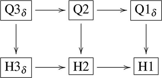
Degeneration relation
4.1. Q3δ −→ Q2
The degeneration from Q3δ to Q2 is implemented through taking
Then, rational solutions for Q2 are given as
Pure rational solutions of Q2 are obtained by taking A = D = 0. The first two of them are
4.2. Q2 −→ Q1δ
To achieve rational solutions for Q1δ, consider degeneration of (4.3) by taking
Meanwhile, we replace the constants appearing in solution (4.3) by
Then the rational solutions for Q1δ can be described as
Some explicit S(a, b) can be seen from (3.56). The first two solutions given by (4.8) are
4.3. Q3δ −→ H3δ
By setting
Let us have a close look at V1(a). Considering S(a, b) defined by (3.52), which is valid for b = −a as well, we find
Since f′[x] is a polynomial of {x1, x3,...,x2N−1}, (see Proposition 2), substituting
When N = 1, V1(a) reads
The first two solutions of H3δ are
4.4. Q2 −→ H2
The degeneration from Q2 to H2 can be obtained by setting
Substituting (4.19) into (4.3), combined with
In the following we derive explicit Casoratian forms for S(0) and S(1). For convenience we take f′ = f′(ϕ′odd(l)). Recalling the analysis for f′ in Sec. 3.3.4, noticing Taylor expansion (3.54) and relation (3.55), we have
Thus, compared with (4.20) and making use of Proposition 1, yield
The case of S(a, a) is little bit complicated. Let
Taking
Then we have
The first two S(0) are
The first two S(1) are
And the first two rational solutions of H2 are
4.5. Q1δ −→ H1
The rational solution to H1 can be obtained from (4.8) through degeneration. Substituting
5. Conclusions
In this paper we have derived solutions in terms of Casoratians for the NQC equation. It turns out that the τ-function f with auxiliary directions (α, β) satisfies the Hirota-Miwa equations that are defined in any three directs of (n, m, α, β), but finally (α, β) are restricted to be (0,0). This indicates that, with regard to generating soliton solutions for the ABS equations (except Q4), the Hirota-Miwa equation acts as a master equation to govern the τ-function f.
Rational solutions of the NQC equation are obtained by considering the case that auxiliary matrices A[ni] take the form (3.25) with k = 0. Such rational solutions can be equivalently derived by taking “long-wave-limit”. In this paper, we examined the significance of our rational solutions in the Miura transformation (2.5) from the NQC equation to Q3δ and in the degenerations from Q3δ to the “lower” equations in the ABS list. As a result, we obtained rational solutions in terms of Casoratians for the NQC equation, Q3δ, Q1δ, H3δ, H2 and H1. However, for Q2 we did not find an explicit form of Z(a, −a) in terms of Casoratians. This will be considered in the future. Besides, it is worthy to mention that {xj} defined through (3.38) play an important role in the analysis of rational solutions.
Compared with [28], one can find that some rational solutions of the ABS equations were obtained by means of Bäcklund transformations in [28] can not be derived in this paper. For example, for the rational solutions of Q1δ, (5.28c) in [28] can not be obtained from (4.8) of the present paper, and vice versa.
A further remark is about solving the NQC equation (2.1). In this paper we solve the equation through solving the system (2.2) that contains the lpKdV equation and two Miura transformations, and is based on the Cauchy matrix scheme that provides many clues for bilinearisation. This system is also used in deriving the Miura transformation (2.5) between the NQC equation and Q3δ (see Appendix A). In some sense, (3.13a–3.13e) can be viewed as a bilinear form of the NQC equation. If we only solve the NQC equation, (2.2a, 2.2b) together with extensions in α-and β-direction are enough (cf. Sec. 9.5.3 in [13]). Note that (2.2a, 2.2b) can be considered as a generalisation (with parameters (a, b)) of the class of Bäcklund transformations investigated in [29] (see (3.1) with (3.5) in [29]). This motivates us to reconsider [29] with parameters, which will be done in the future.
Appendix A. Proof of Theorem 2.1
Proof.
The proof is similar to the one given in Ref. [19]. We need three steps. Let us proceed them step by step.
Step # 1. We first introduce a new associated dependent variable U that is given by:
Lemma A.1.
For u defined in (2.5) and the associated variable U defined in (A.1) the following hold:
Proof.
We denote u and U, respectively, defined by (2.5) and (A.1) as
By adding the four equations in (A.4) and (A.5), we arrive at (A.2a). Similar analysis can be done to (A.2b)–(A.2d).
Step # 2.
Lemma A.2.
The following identities hold
Proof.
We consider the following 2 × 2 matrices:
Evaluating the entries in these matrices we obtain
A similar computation as above yields
Thus, we find that the matrix L in (A.8) can be written as
It remains to compute the determinant of matrix (r(a),
On the other hand, a direct computation of the determinant gives:
Comparing the two expressions for det(L) from (A.13) and (A.14) we obtain the first equation in Lemma A.2.
Step # 3. The last step is by combining the relations (A.2) and (A.6) as well as the lpKdV equation (2.2g) to assert that u solves the Q3δ equation. In fact, multiplying for instance (A.2b) by (A.2d) and using (A.6b), where we identify
Appendix B. Casoratian shift formulae
We list some shift formulae for the Casoratians (3.14), where the basic column vector ϕ(l) satisfies shift relation (3.6) and auxiliary relations (3.9). For convenience, we introduce notations
Acknowledgments
The authors are grateful to the referee for the invaluable comments. This project is supported by the NSF of China (Nos. 11401529, 11301483, 11371241, 11631007) and the NSF of Zhejiang Province (Nos. LY17A010024, LY18A010033).
Footnotes
We keep the variable l in the notation ϕ(l) since Casoratians are defined in terms of shifts in l.
One can consider solitons where we take ϕ1 to be (3.1) and take ϕj (where j ≥ 2) by just replacing k1 with kj in ϕ1. Then we expand kj = k1 + εj at εj = 0 and take limit εj → 0 in the rational forms (3.11) successively for j = 2, 3,...,N. As a result, we get Jordan block solutions. For more details one can refer to [26].
References
Cite this article
TY  - JOUR
AU  - Song-lin Zhao
AU  - Da-jun Zhang
PY  - 2021
DA  - 2021/01/06
TI  - Rational solutions to Q3δ in the Adler-Bobenko-Suris list and degenerations
JO  - Journal of Nonlinear Mathematical Physics
SP  - 107
EP  - 132
VL  - 26
IS  - 1
SN  - 1776-0852
UR  - https://doi.org/10.1080/14029251.2019.1544793
DO  - 10.1080/14029251.2019.1544793
ID  - Zhao2021
ER  -