
Nonautonomous symmetries of the KdV equation and step-like solutions
- DOI
- 10.1080/14029251.2020.1757236How to use a DOI?
- Keywords
- Gurevich–Pitaevskii problem; master-symmetry; Painlevé type equations
- Abstract
We study solutions of the KdV equation governed by a stationary equation for symmetries from the non-commutative subalgebra, namely, for a linear combination of the master-symmetry and the scaling symmetry. The constraint under study is equivalent to a sixth order nonautonomous ODE possessing two first integrals. Its generic solutions have a singularity on the line t = 0. The regularity condition selects a 3-parameter family of solutions which describe oscillations near u = 1 and satisfy, for t = 0, an equation equivalent to degenerate P5 equation. Numerical experiments show that in this family one can distinguish a two-parameter subfamily of separatrix step-like solutions with power-law approach to different constants for x → ±∞. This gives an example of exact solution for the Gurevich–Pitaevskii problem on decay of the initial discontinuity.
- Copyright
- © 2020 The Authors. Published by Atlantis and Taylor & Francis
- Open Access
- This is an open access article distributed under the CC BY-NC 4.0 license (http://creativecommons.org/licenses/by-nc/4.0/).
1. Introduction
The study of solutions of the Korteweg–de Vries equation
Despite these successes, no explicit step-like solutions have yet been found (to the author’s knowledge), similar to solitons in the rapidly decaying case. In fact, it is hardly possible that such a solution can be given by elementary functions or even classical special functions. The goal of the present paper is to show that an answer can be given by some ordinary differential equation of Painlevé type. It should be noted that a similar result was previously obtained by Suleimanov [25] for another Gurevich–Pitaevskii problem, also posed in [12, 13], on the formation of the oscillating zone in the vicinity of the breaking point. The exact answer proposed in [25] was defined as the stationary equation for the linear combination of the 5-th order KdV symmetry and the classical Galilean symmetry, which yields the following ODE consistent with (1.1):
This equation is also one of the representatives of the so-called string equations [18,20]. In general, its real solutions have pole singularities, but there is also a special solution which is regular for all real x and t and has the asymptotic behaviour for |x| → ∞ defined by the equation without derivatives, that is, by the cubic parabola 10u3 + k(6tu + x) = 0. The conjecture on the uniqueness of this solution was formulated in [7] and a rigorous proof of the existence was obtained in [5]. The properties of equation (1.2) and its applications to the Gurevich–Pitaevskii problem were studied in [10, 19, 26, 27].
In this paper we demonstrate, so far only numerically, that the Cauchy problem with the step-like boundary conditions also admits some exact solutions related to nonautonomous symmetries. To this end, we consider the stationary equation for a linear combination of the master-symmetry and the scaling symmetry which is equivalent to some sixth order ODE. Under suitable choice of parameters, this equation admits two different constant solutions which suggests that a regular solution may exist with different asymptotic for x → ±∞. As in the case of the equation (1.2), the difficulty is that the general solutions of this ODE may have singularities, while the regular solutions form a low-dimensional submanifold; so, even their existence is far from obvious.
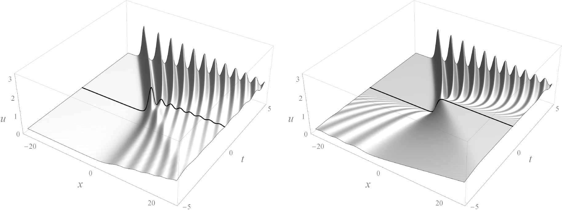
The final result of our experiments is illustrated by Fig. 1, where we compare our solution with the solution of the Cauchy problem with a kink-like initial condition (which is viewed as an approximation of the original Gurevich–Pitaevskii setting with the unit step function). One can see a good agreement for the compression waves, but there are also some peculiar features of our solution which should be noted:
-
— the initial condition is not monotonic;
-
— the approach to limiting values is slow (as O(x−2) for u → 0 and O(x−1) for u → 1);
-
— there are no oscillations in the lower part of the rarefaction wave; instead, there is a slow decay of the initial oscillations in the upper part.
The paper is organized as follows. In section 2 we recall several basic facts about the symmetry algebra of the KdV equation and introduce our sixth order stationary equation (2.1). In section 3 the zero curvature representation is given, based on the well known interpretation of master-symmetry as the flow changing the spectral parameter, see e.g. [2, 4]. This representation provides two first integrals, as well as a more convenient form of equations (3.3), (3.4) which are the main object of further study. In section 4 we discuss, very briefly, a typical scenario of blow-up for the generic solutions of these equations. It should be noted that the efforts in study of Cauchy problems are mainly aimed at the search of the well-posedness conditions, see e.g. [24] where several non-standard settings were discussed. However, the singular solutions are also very interesting, although less studied. Some sufficient conditions for the blow-up of KdV solutions were obtained in [23].
Section 5 contains a description of regular solutions satisfying the fourth order ODE at the special line t = 0 which is the fixed singular line for equations (3.3), (3.4). Taking two first integrals into account, one can reduce this equation to a special case of P5 equation. In turn, this equation has the fixed singular point x = 0 and this effectively lowers the order once again, so that the dimension of regular solutions submanifold is 3. In section 6, we consider the limiting transition to the separatrix solutions at the boundary of this submanifold which finally gives us the desired step-like solutions.
2. Stationary equations for nonautonomous symmetries of KdV
It is well known that the algebra of higher symmetries of the KdV equation is obtained by use of the recursion operator
All flows of order ⩽ 5 read
| ut1 = u1 | (x-translation), |
| ut3 = (u2 + 3u2)x | (t-translation), |
| (higher symmetry), | |
| uτ1 = 6tu1 + 1 | (Galilean transform), |
| uτ3 = 3tut3 + xu1 + 2u | (scaling), |
| uτ5 = 3tut5 + xut3 + 4u2 + 8u2 + 2u1u−1 | (master-symmetry), |
Equation for uτ5 was introduced in [15], see also [4,9,22] for the general notion of master-symmetry. Both sequences ∂ti and ∂τi can be continued infinitely, which gives us the commutative and non-commutative parts of the hierarchy, respectively. However, in this paper we do not need an explicit form of the higher flows. The stationary equation E[u] = 0 for any linear combination of symmetries defines a constraint which is compatible with (1.1) due to the identity
It is well known that the use of only autonomous symmetries leads to the algebro-geometric solutions, and adding any nonautonomous one brings to the Painlevé type equations. For instance, the Suleimanov equation (1.2) is equivalent to ut5 + kuτ1 = 0. Let us take a general linear combination of the flows written above, containing the master-symmetry:
The group of classical symmetries acting on this equation makes possible to fix all the coefficients, which leads to three nonequivalent cases. First of all, we set k3 = k4 = k5 = 0 without loss of generality, by adding constants to t,x and u−1. This gives the equation
Proposition 2.1.
The KdV equation (1.1) and the constraint (2.1) are invariant with respect to the Galilean transformation
It is easy to see that equation
Since we are interested in solutions with different asymptotics for x → ±∞, we will consider only the first case which correspond to the choice
Proposition 2.1 also implies that there is no difference between the right and left step solutions: one is mapped into another under the change x → −x, t → −t. For the sake of definiteness, we will consider the steps with u → 0 as x → −∞. In this case, the compression wave forms for t > 0 and the rarefaction wave forms for t < 0.
3. Zero curvature representation and first integrals
Let us recall the scheme for obtaining the KdV symmetries from linear matrix equations of the form
The symmetries are obtained from the compatibility conditions with the third equation:
One can easily prove that the general form of the matrix W is
Assuming that Y is a polynomial in λ of degree no lower than that of K, we can determine all its coefficients step by step. The stationary symmetry equation has the representation
In the case K = 0 corresponding to autonomous symmetries, equations (3.2) have the common first integral polynomial in λ:
If degY = n then the coefficients of this polynomial give us 2n first integrals which turns out to be enough for the Liouville integrability.
In the case K ≠ 0, only deg K first integrals survive (which is too small to speak about the Liouville integrability), corresponding to the zeroes of K, counting with multiplicities:
In relation to our equation (2.1) with k1 = −4 and k2 = 0, that is, the stationary equation uτ5 −4uτ3 = 0, we have
It is convenient to rewrite the equations in terms of the variables u and y.
Proposition 3.1.
Equations (1.1) and (2.1) with k1 = −4 and k2 = 0 are equivalent to the consistent systems
Equations (3.3) and (3.4) define a pair of non-autonomous dynamical systems with respect to the variables (u,u1, u2, y, y1, y2). The prolongation of the differentiation Dt on u1, u2 and y1, y2 is straightforward: one just has to differentiate equations (3.4) with respect to x, eliminating u3 and y3 by use of (3.3). We omit the resulting equations, since they are rather cumbersome.
Remark 3.1.
The negative flow of the KdV hierarchy is defined by equation
It is easy to see that (3.3) can be interpreted not only as the stationary equation uτ5 − 4uτ3 = 0, but also as the stationary equation uτ3 − 2uτ1 − uτ−1 = 0.
Remark 3.2.
Yet another form of equations is associated with the interpretation of y and z as products of the wave functions of the Schrödinger equation ψ″ +(u +λ)ψ = 0 in the zeroes of K:
Remark 3.3.
Few explicit solutions of equations (3.3), (3.4) are listed in Table 1. The first three solutions are probably the only elementary ones that are regular for all real x and t. In contrast, an infinite sequence of solutions can be obtained from the well known rational solutions of the KdV equation under some special choice of parameters; all these solutions have a real singularity [1]. For instance, the next representative of this family is
| u | y | H0 | H1 |
|---|---|---|---|
| 0 | −2x +a | −4 | −4a2 |
| 1 | a | 4a2 | −4 |
| 2(1 − x tanhX)tanhX, X = x + 4t + a | −4 | −16 | |
| −16 | −4 | ||
| 0 | 0 | 0 | |
| −36 | −16a2 | ||
| 16a2 | −36 |
4. Blow-up of generic solutions
In equation (3.3), the coefficient at the higher derivative u3 is equal to t. Therefore, t = 0 is the fixed singular line for the pair (3.3), (3.4); a generic common solution of these systems acquires a singularity along this line. The explicit solution u = −x/(6t) gives a simplest example of the pole, but, in general, the structure of singularity is much more complicated.
In the half plane t < 0 (or t > 0), the generic solution can be constructed in two ways, given initial data (u0, u1, u2, y0, y1, y2) ∈ ℝ6 at a point (x0,t0), t0 < 0. One way is to solve first the system (3.4) for fixed x = x0. This gives us the initial data for the system (3.3), which we then have to solve for all t ∈ (−∞,0). Another way is to solve first the system (3.3) for fixed t = t0, and then to use the solution as initial data for (3.4), for all x. Both construction methods give the same result due to the commutativity of the flows.
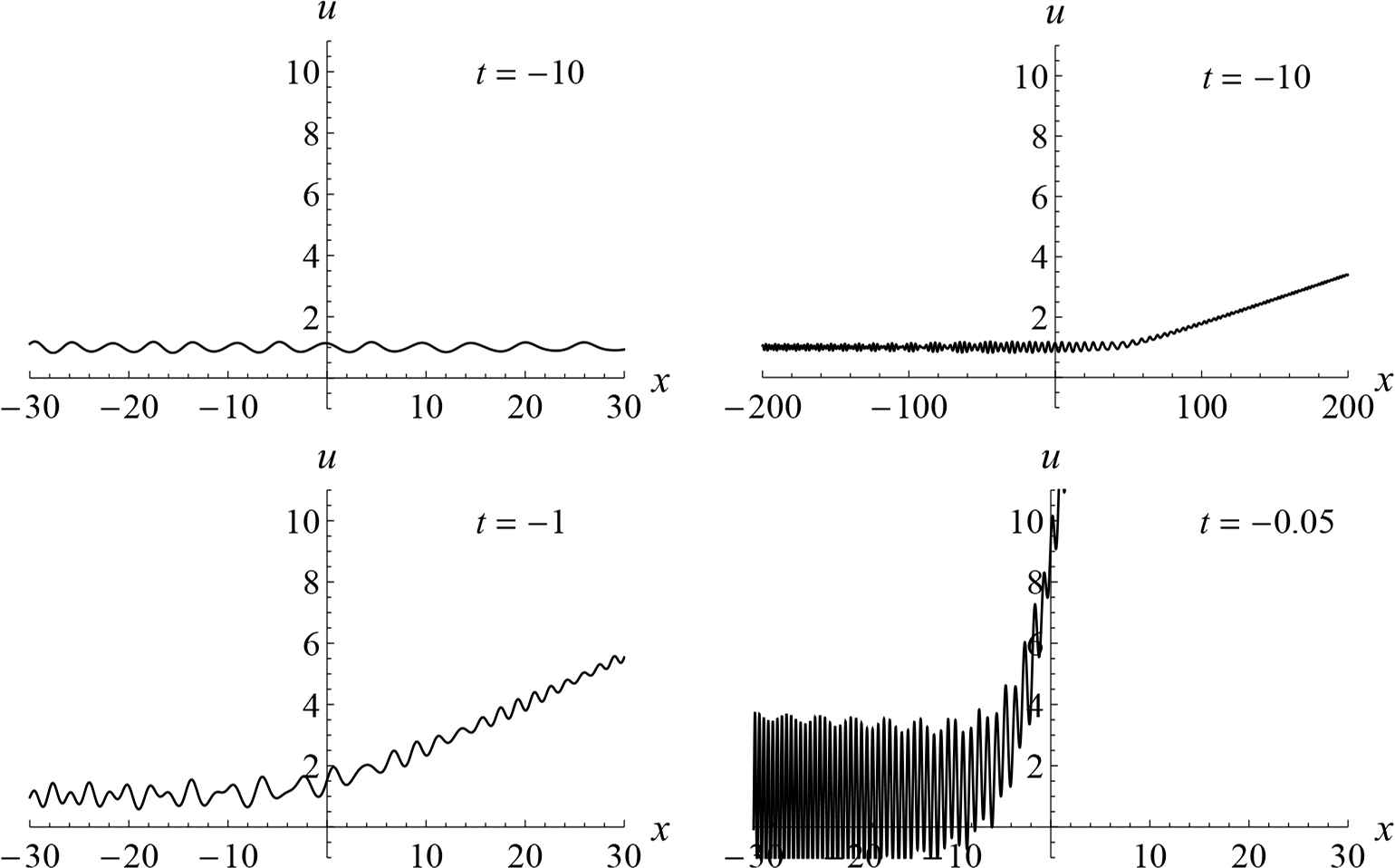
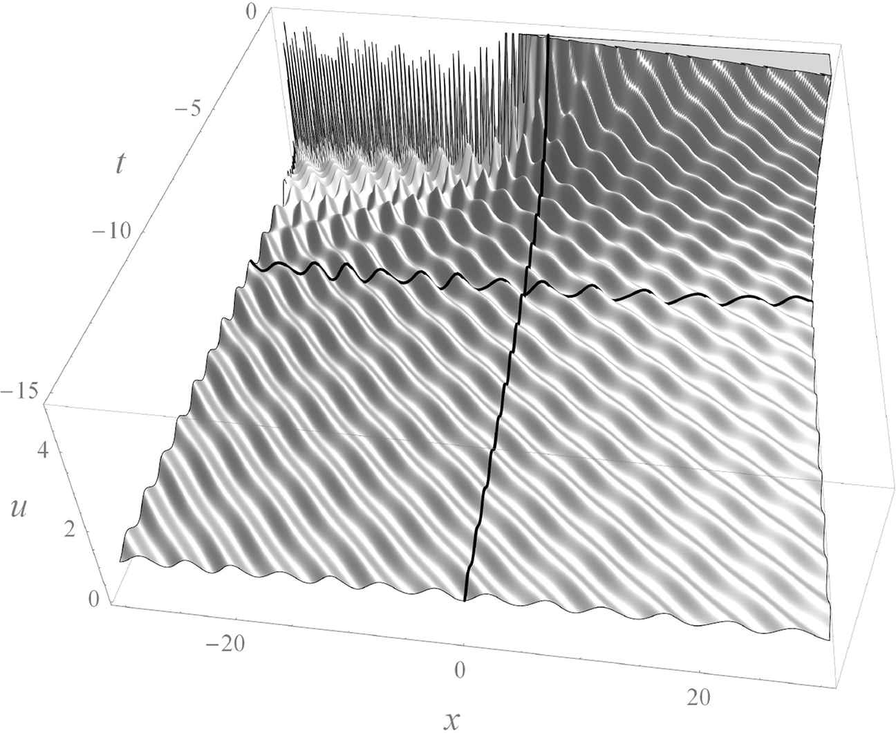
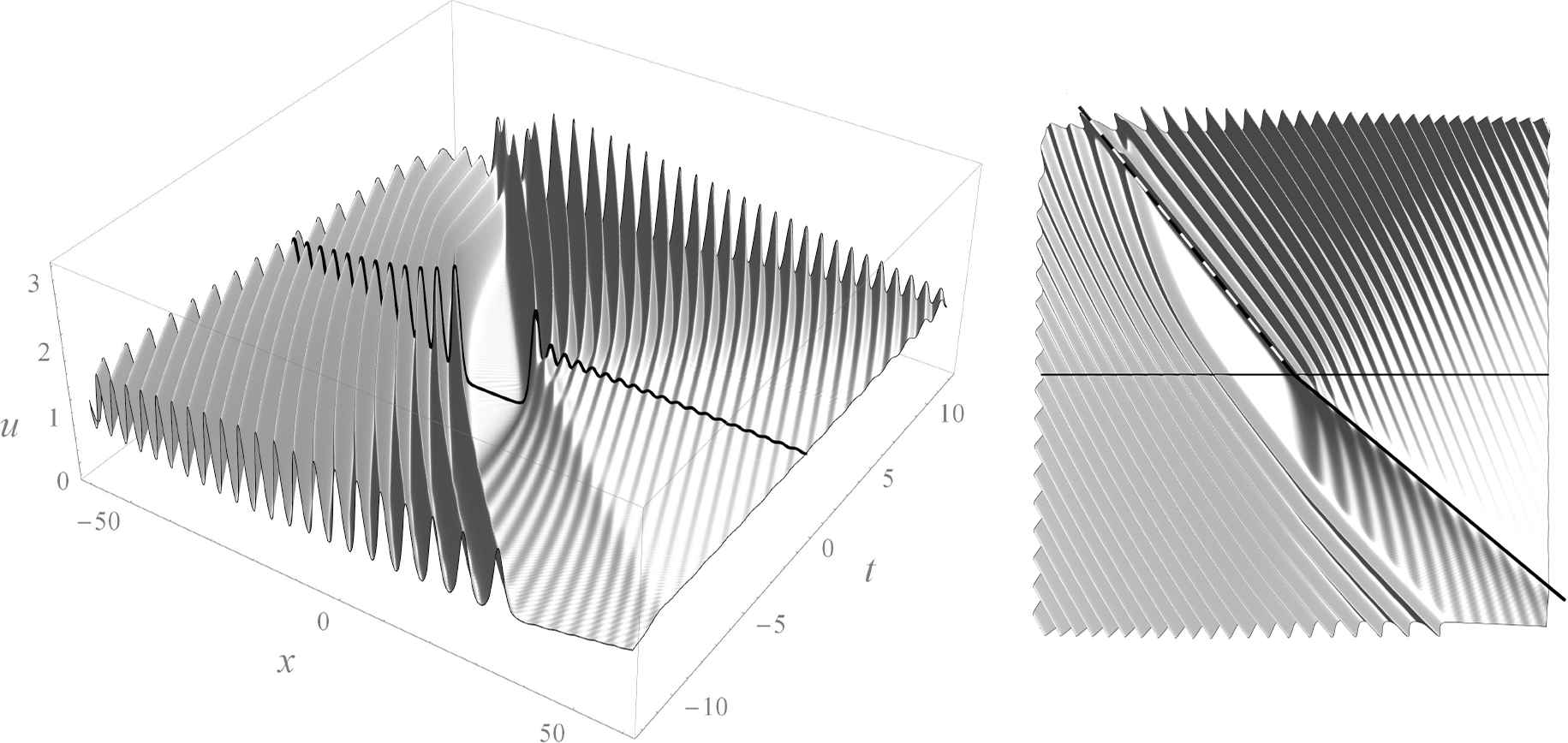
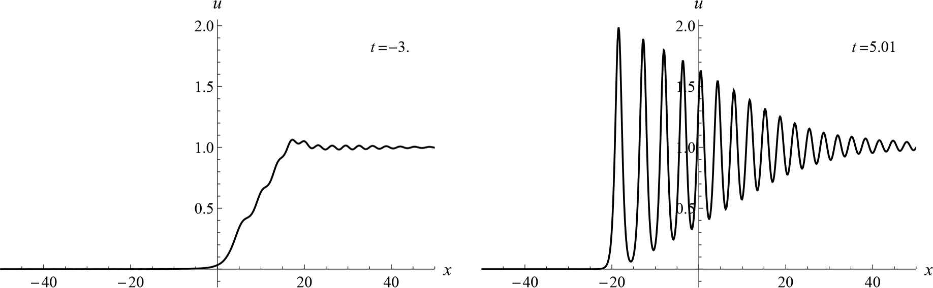
Of course, the constructed solution may have movable poles for t ≠ 0 as well. However, numerical experiments show that for some region in the space of initial data the solutions do not have singularities for x ∈ ℝ and t ∈ ℝ<0 (or t ∈ ℝ>0). For x small enough, a typical solution of such kind looks like small oscillations near u = 1, but, in fact, it grows in x on one half-line (see Fig. 2 where two plots on the top correspond to the same moment t, but have different scales in x). When t increases, the growth in x becomes more noticeable, and at the same time, the amplitude and frequency of oscillations increase on the other half-line. For t → 0 this leads to a pole-like singularity on one half-line and an essential singularity on another, as shown on Fig. 3.
Formation of a singularity at t → 0 for a generic solution.
5. Equation for t = 0 and regular solutions
Further on we consider only special solutions which remain regular for t = 0. For these solutions the order of equation (2.1) on this line lowers and it turns into the fourth order ODE (we assume that k1 = −4 and k2 = 0)
It should be emphasized that the decrease in order occurs only along the special line t = 0; outside it, any regular solution is described by the sixth order equation, as before. The equivalent system (3.3) and its first integrals take the following form, in the prime notation for the derivatives:
This yields the second order equation for y after elimination of u:
It can be brought to the special case of Painlevé equation P5 with vanishing parameter δ [2] which, in turn, is equivalent to a special case of P3 [11].
Proposition 5.1.
The change of variables
System (5.1), in turn, has the fixed singular point x = 0. For solutions that are regular at this point, the initial conditions must be bound by the constraint
Thus, the regularity condition once again lowers the order, from 4 to 3. In a neighborhood of x = 0, regular solutions are constructed in the form of power series
By direct substitution in (5.1), it is easy to prove that a0, a1 and a2 are arbitrary, and all other coefficients are uniquely determined by the recurrence relations
The values of the first integrals, as functions of the inital data, are
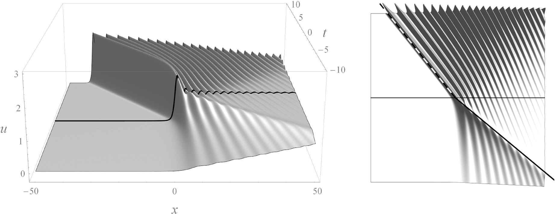
The obtained series have a finite but nonzero radius of convergence and we can use them to construct the solution in some interval near the origin. After this, the solution can be continued numerically by solving equations (5.1) with initial conditions at some point x0 ≠ 0 belonging to this interval. As before, solutions may have movable poles for x ≠ 0, but numerical experiments demonstrate that there exists a domain in the space of initial data (a0, a1, a2) corresponding to solutions which are regular for all real x. A typical regular solution has the form of slowly decaying (like x−1) oscillations near u = 1, separated by a well near the origin, with different oscillation amplitudes on the left and right, see Fig. 4.
Regular solution. Initial profile; view from t < 0; top view, with the half-lines x = −6t, t < 0 and x = −4t, t > 0.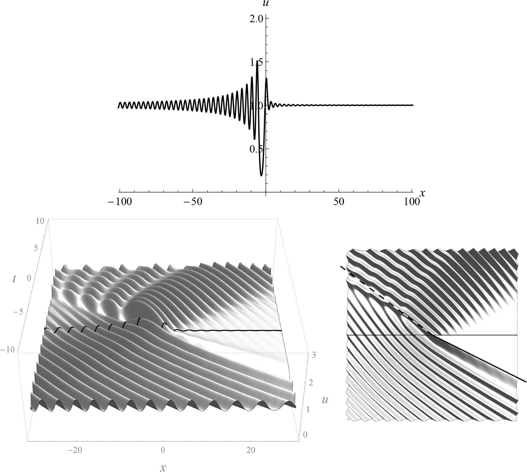
Thus, all regular solutions of our equations are parametrized by the triple (a0, a1, a2) which serves as the initial data at (x,t) = (0,0). Fist, we construct the solution at t = 0 by solving equations (5.1). Next, we have to continue this solution for all t. From the computational point of view, this is the most difficult stage. Theoretically, it also comes down to solving an ODE and can be done in different ways:
-
— by using the solution at t = 0 as the initial data for system (3.4) for all x;
-
— by solving (3.4) for x = 0 only, with the same initial data (a0, a1, a2), and then using the obtained solution as initial data for (3.3) for all t;
-
— by solving equations along the lines x = ct, with initial data (a0, a1, a2).
In practice, all these methods work indeed, but not very well. One of the problems is that the Taylor expansion for system (3.4) is more difficult to construct, and its convergence is worse than for system (3.3). Another problem is that regular solutions are very unstable near t = 0, which is natural, since these solutions form a low-dimensional manifold in the set of generic solutions. On the other hand, given a regular initial condition at t = 0, we can continue it by finite difference methods which turn out, at the moment, to be a more efficient tool.
6. Limiting transition to step-like solutions
By smoothly varying the initial data for the system (5.1), one can notice a broadening of the well near the origin at the moment preceding the formation of a pole. During this elusive moment, the solution remains practically unchanged on one half-axis, but changes drastically on the another one, so that the oscillating zone moves farther and farther from the origin. How far can it be driven away?
Let us use the shooting method to select the initial value y(0) = a0, either for fixed a1,a2 or for fixed values of the first integrals (5.3). Let an interval [a0(1),a0(2)] be given such that the solution corresponding to one endpoint has a pole, and the solution corresponding to another is oscillating. Then we compute the solution at the midpoint and select half the interval so that its endpoints correspond to solutions of different types, as before. Repeating this yields a sequence of values
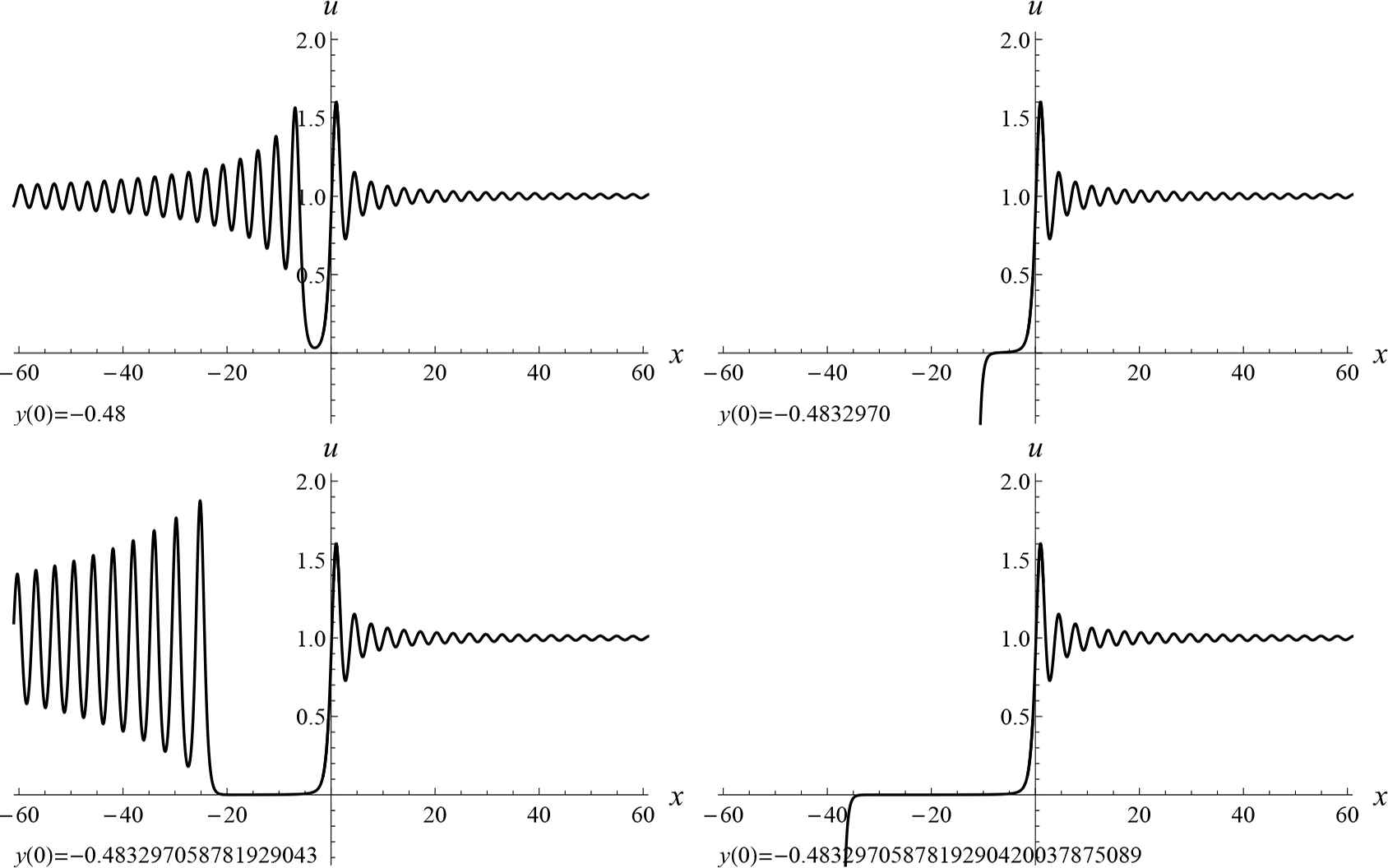
Streching of the step, at H0 = −2, H1 = −6.
Roughly speaking, to expand the well by 1, we need to calculate the next exact decimal digit of a0, which amounts approximately to 3 bisections; and at each step we have to solve the system (5.1) with accuracy no less than the accuracy of a0. Of course, this method is very inefficient and allows us to get only an approximation to the desired step-like solution, with the width of well up to 50. These intermediate solutions are also quite interesting. Continuing them from the initial line t = 0, we can see several typical regions with different oscillation modes, as shown on Fig. 6.
An intermediate solution with a wide well.
A rigorous proof of the existence of step-like solutions for system (5.1) is lacking. A fairly plausible approximation to such a solution can be obtained by taking a well large enough and continuing it by the constant. An example of such approximation is shown on Fig. 7; the structure of the rarefaction and compression waves for this solution are shown on Fig. 8. In accordance to the known asymptotic formulae, the first peak of the compression wave moves parallel to the line x = −4t, t > 0 and the rarefaction wave reaches the unit limiting value along the line x = −6t, t < 0. In these regions the behaviour of solution is determined by the soliton moving at a speed 4, and the singualr solution u = −x/(6t); recall that these are exact solutions of (3.3), (3.4), see Table 1. It is interesting that these lines can be traced down even for general regular solutions, see Fig. 4.
One of step-like solutions for H0 = −2 and H1 = −6. View from t < 0 and top view, with the half-lines x = −6t, t < 0 and x = −4t, t > 0.
The rarefaction and compression waves.
Step-like solutions corresponding to different values of H0 and H1 look more or less similar, but a quantitative difference can be observed at the level of their asymptotic behaviour. The formal asymptotic solution of (5.1) at u → 0 can be found in the form of power series
Thus, the asymptotic behaviour for u → 0 is completely determined by the values of the first integrals. Equations for A2 and B0, and numerical experiments lead us to the following conjecture.
Conjecture 6.1.
Equation (5.1) possesses four step-like solutions for any H0 > −4 and H1 > 0. Two of them have the asymptotic behaviour
7. Conclusion
We have demonstrated that the KdV equation (1.1) admits solutions defined by the pair of ODEs (3.3) and (3.4). For these solutions, the following sequence of degeneracies has been described:
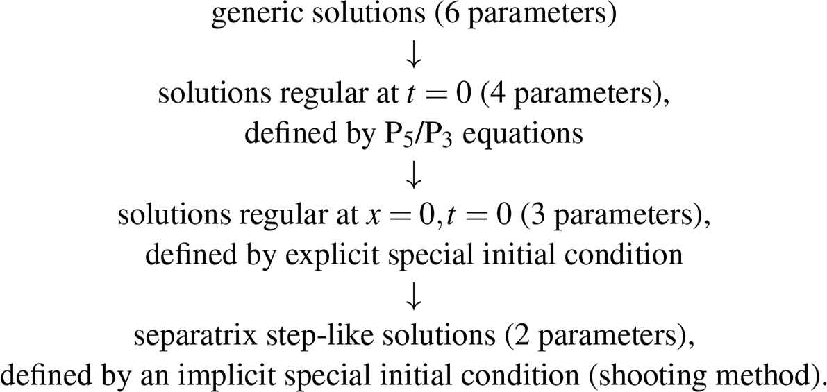
At each stage, the definitions become less effective, which also leads to difficulties in the numerical study. In fact, step-like solutions of (3.3) and (3.4) should be simpler than more general regular solutions (like solitons are simpler than cnoidal waves), but so far we do not know an alternative way to define them. Some open problems are: rigorous proofs of the existence of regular and separatrix solutions; study of their asymptotics and connection formulae; enhancement of numerical schemes; applications to the original Gurevich–Pitaevskii problem and generalizations for other integrable models.
Acknowledgements
I would like to thank A.B. Shabat and B.I. Suleimanov for helpful conversations concerning the Gurevich–Pitaevskii problems. This work was supported in part by the Simons Foundation.
References
Cite this article
TY  - JOUR
AU  - V.E. Adler
PY  - 2020
DA  - 2020/05/04
TI  - Nonautonomous symmetries of the KdV equation and step-like solutions
JO  - Journal of Nonlinear Mathematical Physics
SP  - 478
EP  - 493
VL  - 27
IS  - 3
SN  - 1776-0852
UR  - https://doi.org/10.1080/14029251.2020.1757236
DO  - 10.1080/14029251.2020.1757236
ID  - Adler2020
ER  -