
Group analysis of the generalized Burnett equations
- DOI
- 10.1080/14029251.2020.1757238How to use a DOI?
- Keywords
- Generalized Burnett equations; Lie group; group classification; conservation law; invariant solutions
- Abstract
In this paper group properties of the so-called Generalized Burnett equations are studied. In contrast to the classical Burnett equations these equations are well-posed and therefore can be used in applications. We consider the one-dimensional version of the generalized Burnett equations for Maxwell molecules in both Eulerian and Lagrangian coordinates and perform the complete group analysis of these equations. In particular, this includes finding and analyzing admitted Lie groups. Our classifications of the Lie symmetries of the Navier-Stokes equations of compressible gas and generalized Burnett equations provide a basis for finding invariant solutions of these equations. We also consider representations of all invariant solutions. Some particular classes of invariant solutions are studied in more detail by both analytical and numerical methods.
- Copyright
- © 2020 The Authors. Published by Atlantis and Taylor & Francis
- Open Access
- This is an open access article distributed under the CC BY-NC 4.0 license (http://creativecommons.org/licenses/by-nc/4.0/).
1. Introduction
Symmetries have always attracted the attention of scientists. One of the tools for studying symmetries is the group analysis method [14, 17, 21, 26, 27], which is a general method for constructing exact solutions of partial differential equations. It is worth to mention here that applications of the group analysis method to a wide variety of models in science (up to year 1996) were collected in [16].
The group classification of the viscous gas dynamics equations under some restrictions on the viscosity coefficients was done in [11]. The group classification of two-dimensional steady viscous gas dynamics equations for an ideal gas was done in [22]. For some models of viscous gas dynamics equations, group analysis was applied in [10]. Unsteady two-dimensional steady viscous gas dynamics equations with arbitrary state equations were studied in [23]. Many of the invariant solutions of the viscous gas dynamics equations have also been obtained by other methods [1,2,9,12 ,13,30,33].
In this paper we study symmetry properties of equations of hydrodynamics (derived from the Boltzmann equation) at the Burnett level [15, 20]. This level of description of rarefied gases is important because it includes, for example, physical phenomena such as dispersion of sound waves that are absent at the Navier-Stokes level. However, the well-known instability [4] of the classical Burnett equations makes these equations ill-posed and therefore practically useless for applications. There are several methods to regularize these equations (see, for example, [5,19,32] and references therein). In this paper we use an approach developed by one of the authors, which is based on the idea of ’infinitesimal’ changes of variables. In other words, we consider the equations not for true hydrodynamic variables (density ρtr, bulk velocity vtr, and temperature Ttr), but for slightly different quantities,
This paper is organized as follows. The generalized Burnett equations are introduced and briefly discussed in Section 2. Their group properties are described in Section 3. Section 4 is devoted to invariant solutions. Some non-trivial examples of invariant solutions of the GBEs and their comparisons with invariant solutions of the NSEs are given. The group analysis of the GBEs and NSEs in Lagrangian coordinates is performed in Section 5. Comparisons of invariant solutions in Lagrangian and Eulerian coordinates are presented. Conservation laws are discussed in Section 6.
2. Generalized Burnett Equations
We consider the following set of three equations for density ρ(x,t), bulk velocity v(x,t)= (v(x,t),0,0), and absolute temperature T (x,t) [8]
If the terms with η2 are omitted in (2.2), then equations (2.1) correspond to the Navier-Stokes equations of compressible gas (NSEs).
As always, we set ε = 1 in the resulting equations. The constant positive factor η is given by
equations (1.1) for the GBEs (2.1) read as
We want to make use of this relation. Our aim is to investigate group properties of the GBEs (2.1). This will be done in next two sections.
3. Admitted Lie algebra and its analysis
In this section, group properties of equations (2.1) are studied. We use the standard terminology of group analysis [26, 27], assuming that the reader is familiar with it. Readers who are mainly interested in applications of group analysis such as self-similar solutions, etc., may proceed to the next Section.
3.1. Equivalence group
The first step of the group classification of the class (2.1) is to describe the equivalence among equations from this class, up to which the group classification is carried out.
The class of equations (2.1) is parameterized by the arbitrary element η. Equivalence transformations of the class preserve the structure of its equations, but are allowed to change the arbitrary elements.
Generators of one-parameter groups of equivalence transformations [24, 27] are assumed to be in the form
The class of differential equations (2.1) is defined by auxiliary equations for the arbitrary elements η which are given by
For finding equivalence transformations we have used the infinitesimal criterion [27]. For this purpose the determining equations for the components of generators of one-parameter groups of equivalence transformations were derived. The solution of these determining equations gives the general form of elements of the equivalence algebra of the class (2.1). The basis elements of the equivalence algebra of the class (2.1) are
These generators define the equivalence group of equations (2.1). Because of the transformations corresponding to the generator
For classifying subalgebras of the admitted Lie algebra, one can use the equivalence transformation corresponding to the involution which also an equivalence transformationa
3.2. Admitted Lie algebra
A generator admitted by equations (2.1) is considered in the form
Usual calculations (see e.g. [26, 27]), which are omitted for brevity, show that the admitted Lie algebra L5 is defined by the generators
One notices that
It should be mentioned that the Lie algebra L5 coincides with the Lie algebra admitted by the Navier-Stokes equations of a compressible gas.
Using the commutator table
| X1 | X2 | X3 | X4 | X5 | |
|---|---|---|---|---|---|
| X1 | 0 | 0 | 0 | X1 | X1 |
| X 2 | 0 | 0 | X1 | 0 | X2 |
| X 3 | 0 | −X1 | 0 | X3 | 0 |
| X 4 | −X1 | 0 | −X3 | 0 | 0 |
| X 5 | −X1 | −X2 | 0 | 0 | 0 |
For high-dimensional Lie algebras one can use a two-step algorithm [28]. This algorithm reduces the problem of constructing an optimal system of subalgebras with high dimensions to a problem with low dimensions.
According to the theory of the group analysis method [27], all invariant solutions split into classes of equivalent solutions. The equivalence is considered with respect to the admitted Lie group corresponding to the Lie algebra L5. For finding representatives of these classes one can use an optimal system of the subalgebras of the admitted Lie algebra L5 [27].
The Lie algebra L5 can be presented as the direct sum L5 = L2 ⊕ I3 of the subalgebra L2 = {X4,X5} and the ideal I3 = {X1,X2,X3}. First one construct the optimal system of subalgebras of the subalgebra L2. As the Lie algebra L2 is Abelian, its classification is trivial: an optimal system of one-dimensional subalgebras of the Lie algebra L2 consists of the subalgebras
Here {0} is included in the list for subalgebras which do not include the generators from the Lie algebra L2. The second step consists of joining the ideal I3: each of the elements from the list (3.2) is extended by generators from the ideal I3 using their stabilizer. Finally the optimal system of one-dimensional subalgebras consists of the subalgebras:
4. Representations of invariant solutions
For finding invariant solutions one needs to choose a subalgebra from the optimal system of subalgebras of the admitted Lie algebra (see e.g. [27] for details). Then one finds all functionally independent invariants of the subalgebra. Setting the invariants for which the rank of the Jacobi matrix is equal to the number of the dependent variables by functions of the other invariants, one constructs a representation of a solution invariant with respect to the chosen subalgebra. Substituting the representation of the invariant solution into the original system, one derives a reduced system of equations. Notice that the reduced system of equations has fewer independent variables. Representations of all invariant solutions are presented in Table 1.
| Generator | ρ | v | T | z | |
|---|---|---|---|---|---|
| 1. | X5 + αX4, | t−1R(z), | tαV (z), | t2α Q(z), | xt− (α+1) |
| 2. | X4 + εX2, | R(z), | eεtV(z), | e2εt Q(z), | xe− εt |
| 3. | X5 − X4 − X1, | t−1R(z), | t−1V(z), | t−2Q(z), | x + lnt |
| 4. | X5 + X3, | t−1R(z), | lnt +V (z), | Q(z), | |
| 5. | X2 + X3, | R(z), | t +V (z), | Q(z), | |
| 6. | X2, | R(x), | V (x), | Q(x), | x |
| 7. | X4, | R(t), | xV (t), | x2Q(t), | t |
| 8. | X3, | R(t), | Q(t), | t | |
| 9. | X1, | R(t), | V (t), | Q(t), | t |
Representations of all invariant solutions.
Consider, for example, the subalgebra with the basis generator
For finding invariants J(x,t,ρ,v,T) one should solve the equation
A set of functionally independent solutions of the latter equation can be chosen as follows,
A representation of the invariant solution is
Substituting this representation into equations (2.1), one obtains a system of ordinary differential equations. Because for the GBEs equations these ordinary differential equations are cumbersome, we only present them for the Navier-Stokes equations of compressible gas
Solutions of equations (4.1) and the reduced equations of the GBEs were constructed numerically by a six-th order Runge-Kutta scheme. For testing the code, we used solutions of these systems with V = z and α ≠ 0.
The equation of conservation of mass gives that R′= 0, for example, R = q1, where q1 is constant. Hence, we have only one unknown function Q(z) and two free parameters q1 and α. Note that equations (2.1) in the limiting case η = 0 become the usual Euler equations for monoatomic ideal gas. equations (4.1) for η = 0 and the above assumptions lead to
Thus we have two options:
- (a)
non-trivial limit with
where q2 is constant; - (b)
trivial limit with Q = 0 or/and q1 = 0. Note that the non-trivial limit corresponds to adiabatic solution of the Euler gas dynamic equations
which has clear physical meaning of one-dimensional spatially homogeneous expansion of gas in the whole space. This information is important because we will consider below two different classes of solutions to the NSEs and GBEs.
Case of the NSEs. The remaining equations of the reduced system become
If Q = 0, for example, Q = q2, then equation (4.5) gives that
Then we have two options. If we want to have the non-trivial limit (4.2) at η = 0, we just define a new value of the exponent α
If Q′ ≠0, then
Note that solutions which have trivial limit at η = 0 can be also used as tests for computer codes and numerical methods.
Case of the GBEs. The remaining equations of the reduced system become
If Q = q2, then equation (4.7) gives that
We denote this solution by QGBE = q2 This value of α with free parameters q1 and Q = q2 corresponds to solution of the GBEs, having the non-trivial limit (4.2) at η = 0. Other solutions of (4.6), (4.7) have trivial limit at η = 0. We present here an explicit example of such solution.
If Q′ ≠ 0, then finding Q″ from equation (4.6), integrating it, and substituting into (4.7), one finds that
Numerical solutions of Q of system (4.1) for the NSEs and GBEs are presented in Figures 1–3. For testing the code we used exact solutions obtained above with V (z)= z. Figures 1–2 demonstrate a good agreement of numerical solutions with exact solutions. In Fig. 1 the exact solution is for the NSEs (QNSE), and in Fig. 2 the exact solution is for the GBEs (QGBE). Fig. 3 presents the numerical solution Q of equations (4.1) for the NSEs and GBEs with the following initial data: Q(.5) = 1, R(.5) = 1, Q′(.5) = 10, R′ (.5) = −5, v(.5) = .5. In all these cases the parameter α = −1.852.
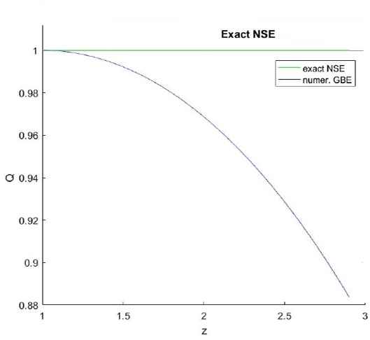
The numerical solution of Q of the NSEs with α = −1.852 coincides with exact constant solution QNSE.
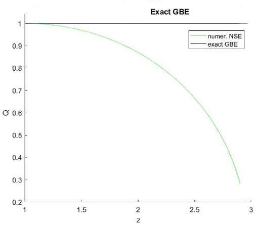
The numerical solution of Q of the GBEs with α = −1.852 coincides with exact constant solution QGBE.
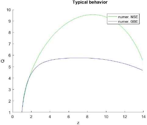
The numerical solution of Q of equations (4.1) with α = −1.852, Q(.5) = 1, R(.5) = 1, Q′(.5) = 10, R′(.5) = −5, v(.5) = .5.
Remark.
Solutions of the travelling wave type were applied in [8] for studying the structure of a shock wave. This type of solution is equivalent to the solution invariant with respect to the generator X2, which corresponds to the set of stationary solutions. The conservative form of equations (2.1) provides three integrals of equations (2.1).
5. Analysis of equations (2.1) in Lagrangian coordinates
The Eulerian (x,t) and mass Lagrangian (ξ, t) coordinates are related by the relation x = φ(ξ, t), where the function φ satisfies the equations
In the mass Lagrangian coordinates (ξ, t) equations (2.1) take the form
5.1. Admitted Lie group
As the transition to the Lagrangian coordinates is not a point transformation, group analysis of these equations has to be performed independently of their representations in Eulerian coordinates. In particular, group classification of the admitted Lie algebra and invariant solutions of equations (2.1) in mass Lagrangian coordinates are obtained in this section.
Calculations show that the admitted Lie algebra
The commutator table is
| Y1 | Y2 | Y3 | Y4 | Y5 | |
|---|---|---|---|---|---|
| Y1 | 0 | 0 | 0 | Y1 | 0 |
| Y2 | 0 | 0 | 0 | 0 | Y2 |
| Y3 | 0 | 0 | 0 | Y3 | 0 |
| Y4 | −Y1 | 0 | −Y3 | 0 | 0 |
| Y5 | 0 | −Y2 | 0 | 0 | 0 |
There is also the involutionb
On the first step one classifies the subalgebra L2 = {Y4,Y5} which is Abelian
Hence, the optimal system of one-dimensional subalgebras of Lie algebra
Representations of all invariant solutions are presented in Table 2. Notice that there are no solutions invariant with respect to Y3.
| Generator | ρ | v | T | z | Tab.1 | |
|---|---|---|---|---|---|---|
| 1. | Y4 + αY5, | t−1R(z), | tαV (z), | t2α Q(z), | ξ t−α | α = −1: X5 − X4 + X1 |
| 2. | Y4 + εY2 | R | ξV | ξ2Q | ξe−εt | α ≠ −1: X5 + αX4 X4 + εX2 |
| 3. | Y5 +Y1 + αY3, | t−1R(z), | V (z) + α lnt, | Q(z), | ξ − lnt | X5 + αX3 |
| 4. | Y1 + Y2 + αY3, | R(z), | V (z) + αt, | Q(z), | ξ−t | X2 + αX3 |
| 5. | Y5 + εY3, | t−1R(z), | V (z) + ε lnt | Q(z), | ξ | X5 + X3 |
| 6. | Y5, | t−1R(z), | V (z), | Q(z), | ξ | X5 |
| 7. | Y2 + εY3, | R(ξ), | V (ξ) + εt, | Q(ξ), | ξ | X2 + εX3 |
| 8. | Y2, | R(ξ), | V(ξ), | Q(ξ), | ξ | X2 |
| 9. | Y1 + αY3, | R(t), | V (t) + α ξ, | Q(t) | t | X1|α=0; X3|α≠0 |
| 10. | Y4 | R | ξV | ξ2Q | t | X4 |
Representations of all invariant solutions.
5.2. Relations between invariant solutions in Lagrangian and Eulerian coordinates
Consider the generator
It has the invariants
A representation of the invariant solution has the form
Hence, the Lagrangian and Eulerian coordinates are related by the formula
Integrating the first equation of (5.3), one has that
Thus, one obtains that
If α + 1 = 0, then h = k ln(t)+ k0, where the constant k0 can be assumed k0 = 0. Hence, one obtains that
Using the inverse function theorem, one obtains that
This is a representation of a solution invariant with respect to the subalgebra X5 − X4 + kX1, which is similar to the subalgebra number 3 in Table 1.
If α + 1 ≠0, then
Using the inverse function theorem, one obtains that
This is a representation of a solution invariant with respect to the subalgebra X5 + αX4, which is number 1 in Table 1.
Representations of all invariant solutions are given in Table 2. Their equivalence with invariant solutions in Eulerian coordinates is presented in the last column of Table 2.
6. Conservation laws
6.1. Eulerian coordinates
In conservative form equations (2.1) are rewritten as
The general form of a conservation law is
Conservation laws provide information on the basic properties of solutions of differential equations, and they are also needed in the analyses of stability and global behavior of solutions. Noether’s theorem [25] is the tool which relates symmetries and conservation laws. However, an application of Noether’s theorem depends on the following condition: that the differential equations under consideration can be rewritten as Euler-Lagrange equations using some Lagrangian. Among approaches trying to overcome this limitation one can mention here the approaches developed in [3,18,29,31 ]c.
In the present paper we use the method applied in [31]. The method consists of substituting the functions Bt and Bx in general form into equation (6.1). Excluding the main derivatives of system (2.1), and splitting it with respect to the parametric derivatives, one derives an overdetermined system of linear partial differential equations for the functions Bt and Bx. The general solution of this system of equations provides the complete set of conservation laws.
The calculations show that the Navier-Stokes equations of a compressible gas only have one additional conservation law
This conservation law can be written in the form
This conservation law in inviscid gas dynamics is called the conservation law of the center of mass. One can check directly that the (
6.2. Lagrangian coordinates
The conservation laws in Eulerian and mass Lagrangian coordinates are related by the formula
The conservation of mass becomes the identity in mass Lagrangian coordinates. The conservation laws of the momentum and energy become, respectively,
The conservation law of the center of mass is reduced to the conservation law of momentum.
7. Conclusions
In this paper we have studied group properties of the so-called Generalized Burnett equations. These equations are well-posed in contrast with the classical Burnett equations, and therefore, are used in various applied problems of rarefied gas dynamics. We considered the one-dimensional version of the GBEs in both Eulerian and Lagrangian coordinates and performed a complete group analysis of these equations. In particular, this includes finding admitted Lie groups and their analysis. The presented classifications of the Lie symmetries of the NSEs and the GBEs provides a basis for finding invariant solutions of these equations. Such solutions can be used for testing numerical schemes for these models. We also considered representations of all invariant solutions. As expected, the complete Lie group and the set of conservation laws are similar for the GBEs and for NSEs. However, there are important differences if we consider some concrete invariant solutions. On one hand, the GBEs are the more accurate equations with respect to the Knudsen number. On the other hand, they contain higher order derivatives and can therefore admit some non-physical solutions. Some classes of invariant solutions were considered in more detail by both analytical and numerical methods. It was shown, in particular, that the GBEs admit two different classes of solutions that can have (a) non-trivial or (b) trivial limits when the mean free path of gas molecule tends to zero. In case (a) the solution tends to the corresponding solution of Euler gas dynamics equations. In case (b) the density of gas tends to zero. This is a natural phenomenon, which shows that higher order PDEs can introduce some ‘spurious’ solutions, which can be removed by boundary conditions, etc. This and other questions related to the GBEs need further investigation and we plan to continue this work.
Acknowledgements
The research was supported by Russian Science Foundation Grant No 18-11-00238 ‘Hydrodynamics-type equations: symmetries, conservation laws, invariant difference schemes’. The authors thank V.A. Dorodnitsyn and E. Schulz for valuable discussions.
Footnotes
The transformation t →−t, v →−v, η →−η does not change the structure of equations (2.1) either.
There is also the involution t →−t, v →−v η →−η.
Therein one can find more details and references.
References
Cite this article
TY  - JOUR
AU  - Alexander V. Bobylev
AU  - Sergey V. Meleshko
PY  - 2020
DA  - 2020/05/04
TI  - Group analysis of the generalized Burnett equations
JO  - Journal of Nonlinear Mathematical Physics
SP  - 494
EP  - 508
VL  - 27
IS  - 3
SN  - 1776-0852
UR  - https://doi.org/10.1080/14029251.2020.1757238
DO  - 10.1080/14029251.2020.1757238
ID  - Bobylev2020
ER  -