
Global dynamics of a Lotka–Volterra system in ℝ3
- DOI
- 10.1080/14029251.2020.1757240How to use a DOI?
- Keywords
- Lotka–Volterra system; phase portraits; Poincaré ball
- Abstract
In this work we consider the Lotka–Volterra system in ℝ3
introduced recently in [7], and studied also in [8] and [14]. In the first two papers the authors mainly studied the integrability of this differential system, while in the third paper they studied the system as a Hamilton-Poisson system, and also started the analysis of its dynamics. Here we provide the global phase portraits of this 3-dimensional Lotka–Volterra system in the Poincaré ball, that is in ℝ3 adding its extension to the infinity.- Copyright
- © 2020 The Authors. Published by Atlantis and Taylor & Francis
- Open Access
- This is an open access article distributed under the CC BY-NC 4.0 license (http://creativecommons.org/licenses/by-nc/4.0/).
1. Introduction and statement of the main results
The Lotka–Volterra systems, developed independently by Alfred J. Lotka in 1925 [9] and Vito Volterra in 1926 [15], were initially proposed as models for studying the interactions in two dimensions between species. Kolmogorov [5] in 1936 extended these systems to arbitrary dimension and degree, which are now called Kolmogorov systems.
The Lotka–Volterra systems have been applied to model different natural phenomena such as the time evolution of conflicting species in biology (which began with the work of May [10]), the evolution of competition between three species (studied by May and Leonard [11]), the evolution of electrons, ions and neutral species in plasma physics [6], chemical reactions [4], hydrodynamics [1], economics [13], etc.
In this work we consider the following Lotka–Volterra system
The main goal of this work is to describe the global dynamics of the Lotka–Volterra system (1.1) in ℝ3 adding the infinity, i.e. we are interested in describing the phase portraits of system (1.1) on the Poincaré ball 𝔻3. A first attempt to describe these phase portraits was done in [14] where the authors gave a Hamilton-Poisson formulation of system (1.1). Leach and Miritzis in [7] proved that system (1.1) has a first integral, and in [8] the authors proved that this system has the two independent first integrals x(y − z) and y(z − x). The existence of these first integrals has some consequences on the phase portrait of the system. Thus on the invariant plane x = 0 one gets that all trajectories are contained in the hyperbolas yz = constant. On the other hand, a generic trajectory is contained in the elliptic curves intersection of the surfaces x(y − z) = constant and y(z − x) = constant. In any case these informations are not sufficient for obtaining the global phase portrait of system (1.1) in the Poincaré ball.
Our objective is to establish the α- and ω-limit of all the orbits of system (1.1) and to characterize the phase portrait of this system in the Poincaré ball 𝔻3. We recall that the Poincaré ball can be seen as the closed unit ball centered at the origin of ℝ3, where its interior is identified with ℝ3 and its boundary 𝕊2 is identified with the infinity of ℝ3 (in the sense that in ℝ3 we can go or come from infinity in as many directions as points has the 2-dimensional sphere 𝕊2).
A polynomial differential system in ℝ3 (in the interior of 𝔻3) can be extended analytically to its boundary 𝕊2. This extension was done by the first time by Poincaré in [12] for polynomial differential systems in ℝ2 and it is called the Poincaré compactification. In [2] the authors give an extension to polynomial differential systems in ℝ3. For a brief introduction to Poincaré compactification see the appendix.
Two compactified polynomial differential systems in the Poincaré ball 𝔻3 are topologically equivalent if there is a homeomorphism of 𝔻3 which send orbits of one system into orbits of the other system, preserving or reversing the orientation of all orbits.
We note that system (1.1) has the symmetry (x,y,z,t) → (−x,−y − z,−t). Then it is sufficient to study its dynamics for x ≥ 0.
In the next theorem we describe the phase portrait on the half-ball x ≥ 0 of the Poincaré ball for the 3-dimensional Lotka–Volterra system (1.1).
Theorem 1.1.
The dynamics of the 3-dimensional Lotka–Volterra system (1.1) in the Poincaré ball is the following.
- (a)
- (b)
The phase portraits on the invariant planes x = z, y = z and x = y are shown in Figure 3.
- (c)
The phase portrait at infinity is topologically equivalent to the one of Figure 4.
- (d)
The phase portraits on the boundary of the twelve invariant regions obtained dividing the Poincaré ball by the six previous invariant planes in the region x ≥ 0 are topologically equivalent to the ones shown in Figure 6.
- (e)
The paper is organized as follows. In section 2 we study system (1.1) on the planes x = 0, y = 0, z = 0, y = x, z = y and z = x, and we prove statements (a) and (b) of Theorem 1.1. In section 3 we study the infinite equilibria of system (1.1) and give the phase portraits on the Poincaré ball, proving statements (c), (d) and (e) of Theorem 1.1. In the appendix there is a brief description of the Poincaré compactification for polynomial differential systems in ℝ3 and in ℝ2.
2. Phase Portraits of system (1.1) on the planes
In this section we study all the phase portraits of the 3-dimensional Lotka–Volterra system (1.1) on the planes x = 0, y = 0, z = 0, y = x, z = y and z = x.
First we point out that in [8] the authors proved that system (1.1) has the two independent first integrals
Moreover the unique irreducible Darboux polynomials with non-zero cofactor of system (1.1) are:
- (1)
x, y, z with cofactors −(x − y − z), −(−x + y + −z), and −(−x + −y + z), respectively.
- (2)
x − z, y − z and z − x with cofactors −(x − y + z), −(−x + y + z), and −(x + y − z), respectively.
We separate the study of the dynamics in the invariant planes in two cases.
2.1. Phase portraits on the invariant planes x = 0, y = 0 and z = 0
First note that system (1.1) on the planes x = 0, y = 0 and z = 0 are equivalent. In fact, system (1.1) on x = 0 is given by
Clearly system (2.1) and system (2.2) are equivalent through the change of variables (y,z) → (x,z), and system (2.3) is equivalent to the previous ones considering the changes of variables (x,y) → (x,z), or (x,y) → (y,z) to get system (2.2), or (2.1), respectively. Hence we are only going to analyze the global phase portraits of system (2.3).
We start with the study of the infinite singular points. For this purpose we use the Poincaré compactification of a polynomial differential systems in ℝ2, see details in chapter 5 of [3]. System (2.3) in the local chart U1 is given by
From systems (2.4) and (2.5) we get that at infinity (i.e. at all points having the coordinate z2 = 0) the origin of each chart is an equilibrium point. Moreover, in U1 we have a second equilibrium point given by (1,0). The eigenvalues of the linear part at the origins of U1 and U2 are 1 and 2, so they are unstable nodes. Note that since system (2.3) has degree 2 the corresponding equilibria on V1 and V2 will be stable nodes. The equilibrium (1,0) in U1 is not a hyperbolic equilibrium. It is at the infinity of the straight line x = y which is filled of equilibria as will be seen later on in the next.
Now we study the finite singular points. System (2.3) has a straight line of equilibria given by x = y. Since −x + y is a common factor of system (2.3), doing a reparametrization of the time, system (2.3) becomes
It is known that the global dynamics of system (2.6) is the following: it has a saddle at the origin with stable separatrices on the y-axis and unstable separatrices on x-axis and at infinity it has infinite unstable nodes at the origins of U1 and V1 and infinite stable nodes at the origins of U2 and V2.
Going back through the reparametrization of time, taking into account the change of stability in the region −x + y < 0 and the straight line of finite equilibria on −x + y = 0, we can complete the global phase portrait of system (2.3) by using the Poincaré Bendixson Theorem (see [3]) connecting the separatrices of the saddle at the origin to the nodes at the infinity. Doing so we obtain the phase portrait described in Figure 1(a).
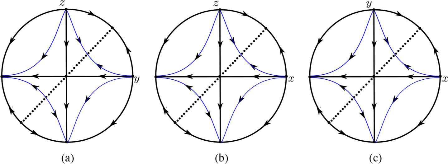
Phase portraits of system (1.1) in the planes x = 0, y = 0 and z = 0, respectively.
The phase portraits in the planes x = 0, y = 0 and z = 0 in ℝ3 are shown in Figure 2. This completes the proof of statement (a) of Theorem 1.1.
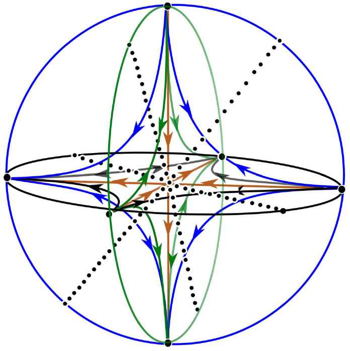
Phase portrait of system (1.1) on the planes x = 0, y = 0, z = 0 inside the Poincaré ball.
2.2. Phase portraits on the invariant planes x = z, y = z and y = x
Note that the dynamics of system (1.1) restricted to the plane x = z, to the plane y = z and to the plane y = x are topologically equivalent. Actually it is sufficient to study the phase portrait in the plane x = z (taking z → x) and inthis case system (1.1) takes the form
System (2.7) has the common factor y. Eliminating this common factor by reparametrizing the time, it becomes
At infinity we have that system (2.8) in the local chart U1 is
The origin is an equilibrium point which is an unstable node. The same stability has the origin of V2. Observe that system (2.7) has the opposite stability in the region y < 0 than system (2.8).
From the previous analysis of system (2.8), considering the reparametrization done with the factor y, and due to the fact that there are not more finite equilibria, by the Poincaré Bendixson Theorem, we have that the separatrices of the saddle at the origin connect with the nodes at infinity. We can thus conclude that the phase portrait in the Poincaré disc of system (2.7) is the one described on Figure 3. Statement (b) of Theorem 1.1 has been proved.
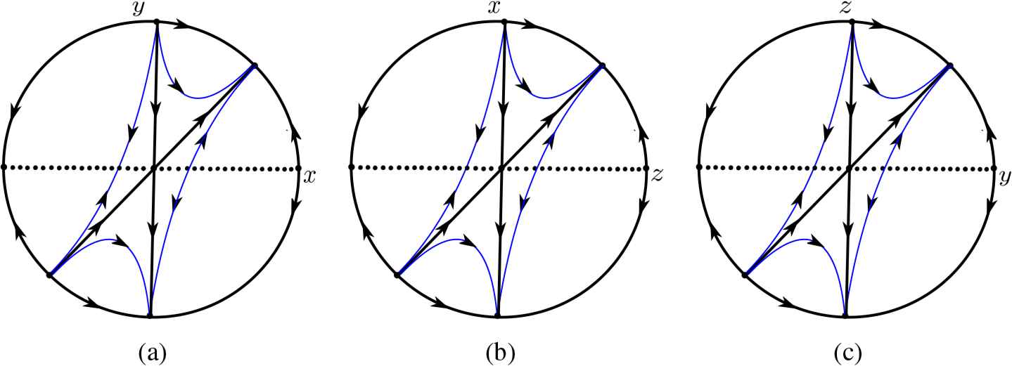
Phase portraits of system (1.1) in the planes z = x, y = z and x = y, respectively.
3. Dynamics on ℝ3
In order to obtain the phase portrait in ℝ3 of system (1.1) we first study the phase portrait at infinity using the Poincaré compactification (for details of the Poincaré compactification in ℝ3, see appendix A.1).
System (1.1) in the local charts U1, U2 and U3 are exactly the same, except for the meaning of the coordinates (z1,z2,z3) (see (A.1), (A.2) and (A.3)). At infinity we have the following system in the local charts
Considering (3.1) on the local chart U1, we have the four infinite equilibria (i.e, on z3 = 0): the origin,
All the infinite equilibria are at the infinity of the planes studied in section 2 and so their phase portraits are known. Due to the fact that the linear part of system (3.1) is
In summary in the Poincaré ball we have 14 infinite equilibria. They are p1 = (1,0,0), p2 = (1,1,0), p3 = (1,0,1), p4 = (1,1,1), p5 = (0,1,0), p6 = (0,1,1) and p7 = (0,0,1) on the charts U1,U2 and U3 and their corresponding antipodal equilibria on the local charts Vi (that we will denote by qi the antipodal point of pi) for i = 1,2,3.
Using the Poincaré-Bendixson Theorem we can characterize the connections between the separatrices of the saddles at p2, p3 and p6 with the infinite nodes. Furthermore, these separatrices are on the invariant planes studied in section 2. The phase portrait at infinity is the one shown in Figure 4. This completes the proof of statement (c) of Theorem 1.1.
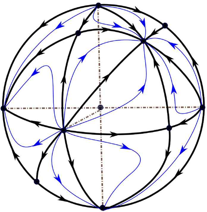
Phase portrait of system (1.1) at infinity on the boundary of the Poincaré ball for x ≥ 0.
On the other hand, the finite equilibria of system (1.1) are the origin and the straight lines of equilibria already mentioned in section 2. Then we can describe the phase portrait in the Poincaré ball.
In order to give an efficient description of the global dynamics of system (1.1) we separate the Poincaré ball in regions defined by the intersections of the planes x = 0, y = 0, z = 0, x = y, x = z and y = z. There are 24 regions, all invariant by the flow of system (1.1). Due to the symmetry (x,y,z,t) → (−x,−y,−z, −t) it is sufficient to analyze the invariant regions contained in x ≥ 0. These regions are
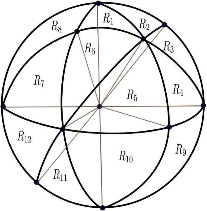
Regions R1 − R12 on the Poincaré ball.
To provide the phase portrait in each of these regions we describe first the phase portrait in the faces of each region, and after that the phase portrait in the interior of them. Note that in each region the isolated equilibria are on the vertices of the region and a segment filled of equilibria is on an edge of the region. We recall that one orbit in each face and one orbit in the interior are sufficient for determining the phase portraits in each invariant region. The edges of the regions are separatrices or segments filled of equilibria.
As an example we consider the region R1. This region is a tetrahedron formed by three infinite equilibria p3, p4 and p7 and the finite equilibrium at the origin θ. Note that it has one edge, given by x = z and y = 0, which connects the vertex p3 with θ filled of equilibria. The infinite equilibrium p4 is an attractor and p7 is a repeller. By the Poincaré-Bendixson Theorem we can establish the α- and ω-limits of all the orbits in this region.
In the faces of R1 without a segment filled of equilibria all the orbits have their ω-limit in p4 and their α-limit in p7.
On the face formed by p3, p7 and θ the orbits have their α limit in p7 and the ω-limit on the edge filled of equilibria.
On the face formed by p3, p4 and θ all orbits have their ω-limit at p4 and their α-limit on the edge filled of equilibria.
Finally in the region R1, by the Poincaré-Bendixson Theorem, we can conclude that an orbit in the interior of R1 has its α-limit at p7 and its ω-limit at p4.
The phase portrait in the remaining regions can be characterized analogously. In Table 1 it is shown the α- and ω-limits for all orbits in the interior of each region.
| R1, R2 | R3, R4 | R5, R6 | R7, R12 | R8 | R9 | R10, R11 | |
|---|---|---|---|---|---|---|---|
| α-limit | p7 | p5 | p1 | p1 | p7 | p5 | p1 |
| ω-limit | p4 | p4 | p4 | q5 | q5 | q7 | q7 |
α- and ω-limits in the interior each invariant region R1-R12.
In Figure 6 it is shown the phase portraits on the boundary of the invariant regions, and one orbit in the interior of each invariant region is shown in Figure 7. These previous results prove statements (d) and (e) of Theorem 1.1 and complete the proof of Theorem 1.1.
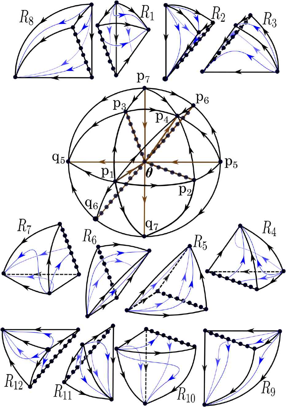
Phase portraits of system (1.1) at the boundaries of the 12 regions contained in x ≥ 0 obtained dividing the Poincaré ball by the six invariant planes, x = 0, y = 0, z = 0, x = y, x = z and y = z.
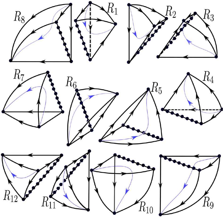
Phase portraits of system (1.1) in the interior of the invariant regions.
A. Poincaré Compactification
We give a description of the Poincaré compactification in order to describe the phase portraits in the Poincaré ball. The Poincaré compactification of ℝ3 is needed in the proof of Theorem 1.1.
We consider a polynomial vector field 𝒳 = (P,Q,R) associated to the polynomial differential system
Now we shall describe the equations of the Poincaré compactification of a polynomial differential system in ℝ3.
We consider the local charts (Uk,φk) and (Vk,ψk) for k = 1,2 on the disc 𝔻3 defined by
Note that the coordinates (z1,z2,z3) have different meaning depending on local chart, but the points at infinity, i.e. the points of the boundary 𝕊2 of 𝔻3 have all the coordinate z3 = 0.
Now we give the expression of the compactified vector field p(𝒳) of the polynomial vector field X = (P,Q,R) in each local chart. The expression of the compactified analytical vector field p(𝒳) of 𝒳 of degree n on the local chart U1 of 𝔻3 is
In a similar way the expression of p(𝒳) in U2 is
Finally the vector field p(𝒳) in U3 is
The singular points of p(𝒳) which are on the boundary 𝕊2 of 𝔻3 (at z3 = 0) are called infinite singular points, and we call finite singular points the ones which are in the interior of 𝔻3.
From equations (A.1), (A.2) and (A.3) it follows that the infinity 𝕊2 of the Poincaré ball is invariant under the flow of the compactified vector field p(𝒳). For studying its infinite singular points we only need to study the ones that are on the local chart U1, in U2 with z1 = 0, and the origin of the local chart U3 in case that this is a singular point.
The expression for p(𝒳) in the local chart Vk is the same as in Uk multiplied by (−1)n−1. Therefore the infinite singular points appear on pairs diametrally opposite on 𝕊2 with the same stability if n is odd and with the opposite stability if n is even. For more details on the Poincaré compactification in ℝ3 see [2].
As we said in the introduction two compactified polynomial differential systems in the Poincaré ball 𝔻3 are topologically equivalent if there is a homeomorphism of 𝔻3 sending orbits of one system to orbits of the other system, either preserving or reversing the orientation of the orbits.
Acknowledgements
We thank to the reviewer his/her good comments which help us to improve the presentation of our results.
The first author is partially supported by the Ministerio de Economía, Industria y Competitividad, Agencia Estatal de Investigación grants MTM2016 - 77278 - P (FEDER) and MDM - 2014 - 0445, the Agència de Gestió d’Ajuts Universitaris i de Recerca grant 2017SGR1617, and the H2020 European Research Council grant MSCA-RISE-2017-777911.
The second author is supported by CONICYT PCHA / Postdoctorado en el extranjero Becas Chile / 2018 - 74190062.
The third author is partially supported by FCT/Portugal through UID/ MAT/ 04459/2013.
References
Cite this article
TY  - JOUR
AU  - Jaume Llibre
AU  - Y. Paulina Martínez
AU  - Claudia Valls
PY  - 2020
DA  - 2020/05/04
TI  - Global dynamics of a Lotka–Volterra system in ℝ³
JO  - Journal of Nonlinear Mathematical Physics
SP  - 509
EP  - 519
VL  - 27
IS  - 3
SN  - 1776-0852
UR  - https://doi.org/10.1080/14029251.2020.1757240
DO  - 10.1080/14029251.2020.1757240
ID  - Llibre2020
ER  -