
Hierarchies of q-discrete Painlevé equations
current email: halrashidi@ksu.edu.sa
- DOI
- 10.1080/14029251.2020.1757235How to use a DOI?
- Keywords
- q-discrete Painlevé equations; Lax pair; Hierarchies; Bäcklund transformations
- Abstract
In this paper, we construct a new hierarchy based on the third q-discrete Painlevé equation (qPIII) and also study the hierarchy of the second q-discrete Painlevé equation (qPII). Both hierarchies are derived by using reductions of the general lattice modified Korteweg-de Vries equation. Our results include Lax pairs for both hierarchies and these turn out to be higher degree expansions of the non-resonant ones found by Joshi and Nakazono [29] for the second-order cases. We also obtain Bäcklund transformations for these hierarchies. Special q-rational solutions of the hierarchies are constructed and corresponding q-gamma functions that solve the associated linear problems are derived.
- Copyright
- © 2020 The Authors. Published by Atlantis and Taylor & Francis
- Open Access
- This is an open access article distributed under the CC BY-NC 4.0 license (http://creativecommons.org/licenses/by-nc/4.0/).
1. Introduction
Following widespread interest in the Painlevé equations, it is natural to ask whether their integrable discrete versions share their fundamental properties. In this paper, we consider and answer the following question about multiplicative or q-discrete Painlevé equations, namely the construction of new associated infinite sequences of discrete equations called hierarchies. The term ‘hierarchy’ here refers to a sequence of q-difference equations sharing a linear problem.
In the literature, discrete hierarchies are known for some additive discrete Painlevé [10,16], and q-discrete Painlevé equations [21,32,45] but not for most of the known discrete Painlevé equations. Our paper extends the class of known hierarchies of q-discrete Painlevé equations by providing a new hierarchy, associated with the q-discrete third Painlevé equation.
Our approach starts with an integrable partial difference equation, also known as a lattice equation, and considers higher-order reductions than those that have been constructed before. (See for example [19, 25, 34, 37–39].) Our starting point is equation (3.1), which is a slightly more general (multi-parameter) form of a standard lattice equation denoted by
In particular, we obtain two q-discrete hierarchies, whose starting points are the q-discrete second and third discrete Painlevé equations, denoted by qPII and qPIII respectively below. We will refer to the nth member of the respective hierarchies by
For Equations (1.1a) and (1.1b) to be compatible, we must have
For each n ∈ ℕ corresponding to the degree of A in x, we show that equation (1.2) gives rise to either
Previous approaches [10, 21] for constructing hierarchies have started by extending the degree of the matrix A in x and using the resulting compatibility conditions to derive new equations. The key idea here relies on fixing one matrix while we change the degree of the other one. However, the calculations are not straightforward, and become more technical in the case of q-discrete equations. Instead, we pursue a simpler approach given by higher-order reductions of systems of lattice equations, as explained in Section 3. In finding the appropriate reductions, we were motivated by the Lax pairs and the actions of the time-deformation operator 𝒯 on parameters given in [29], which allow us to hypothesize the lattice parameters that we use for the reductions.
Given an integer d, a well-known procedure for finding reductions of lattice equations governing a function x(l,m) is to assume a periodic (d,1)-reduction, i.e., impose xl,m+1 = xl+d,m or xl,m+1 = 1/xl+d,m. Such periodic reductions of the lattice mKdV (modified Korteweg-de Vries) equation, also known as H3, were obtained for some integer d in [21]. We note that this led to a qPII hierarchy, which we also find here. However, the calculations are intricate and further assumptions were required to find Lax pairs. In contrast, our approach immediately provides hierarchies as well as their Lax pairs, without intermediate assumptions.
The 2 × 2 Lax pairs we find have certain advantages for analysis. The most important properties are that each matrix A corresponding to a member of the hierarchy is non-singular at x = 0 and ∞ and explicitly factorisable into linear factors in x. The former property enables Birkhoff and Carmichael’s classical theory of non-resonant q-linear difference equations [6, 9] to be applied immediately.
1.1. Background
In this section, we provide some background material about Painlevé and discrete Painlevé equations, and integrable lattice equations.
The Painlevé equations appear widely in physical applications (see for example [46]). They were discovered originally by Painlevé [40], Gambier [14] and Fuchs [13] in the search for new transcendental functions that satisfy ordinary differential equations (ODEs) and their general solutions are known to be higher transcendental functions, called the Painlevé transcendents. Later, they were found as reductions of completely integrable partial differential equations (PDEs), such as the Korteweg-de Vries equation [1, 2]. More recently, integrable difference equations with properties that are very similar to those of the classical Painlevé equations have been identified. They are now known as discrete Painlevé equations and there are three types. We focus here on discrete Painlevé equations of q-discrete or multiplicative type; see Sakai [43].
The search for discrete versions of integrable PDEs has also been a very active area of recent research. Many partial difference equations with properties that are very similar to those of integrable PDEs are known to share a geometric property called consistency around a cube (CAC) or multi-dimensional consistency [35,36]. Classifications of scalar equations with this property [3,4,7] led to a list of scalar partial difference equations. By convention, they are denoted as A-, D-, H- or Q-type. In this paper, we focus on an example of H-type, denoted H3, which is also known as a lattice mKdV equation.
Many reductions of lattice equations to the q-discrete Painlevé equations are already known [8, 12, 19, 22, 23, 26, 34, 37–39]. For example, the qPII and qPIII equations were derived from a so-called geometric reduction of H3 and a special case of an equation labelled D4 in [7]; see [30].
Motivated by the existence of hierarchies (infinite sequences) of PDEs associated with each integrable PDE, hierarchies of Painlevé equations have also been found [15, 28]. Correspondingly, hierarchies for a restricted set of discrete Painlevé equations have also been obtained [10, 21, 33]. However, to the best of our knowledge, very few q-discrete Painlevé hierarchies have been constructed.
Although generic solutions of discrete Painlevé equations are higher transcendental functions, there also exist special function and rational solutions for special cases of parameters. Each such special-parameter case can be mapped to another through transformations called Bäcklund transformations [24]. Explicit solutions of qPII were studied and corresponding solutions of its Lax pair found in [31].
Starting with a seed solution corresponding to an initial parameter, one can generate an infinite series of solutions of the same equation with different parameters, provided that the Bäcklund transformation we use does not terminate. Confusingly, the word hierarchy may also be used in this context to refer to an infinite sequence of solutions generated by a Bäcklund transformation when successively applied to a seed solution.
1.2. Main Result
Our main result shows that each member of the hierarchy of qPII and qPIII shares one spectral linear problem equation (1.1a), with the coefficient matrix given by
Here, bl, l = 0,1,...,n, λand q are the non-zero complex parameters and hl, l = 0,1,...,n are dependent variables. We find that the product of all hl turns out to be constant in the case of the qPII and qPIII hierarchies. We take this constant to be λ 2 without loss of generality, to match with the second-order case given in [29], that is,
We also take
We use the following notation. Given 2 ⩽ n ∈ ℕ, the nth member of the hierarchy will be described by using a deformation operator referred to as
The following theorem collects our main results.
Theorem 1.1
Let n ∈ ℕ, n ≥ 2. The compatibility condition (1.2) is satisfied on solutions of the qPII and qPIII hierarchy respectively when {𝒯, B} is replaced by one of the following choices:
(1) {
- (1)
Take
and defineThen the resulting hierarchy of equations is given by
- (2)
Take
and defineThen the resulting hierarchy of equations is given by
Remark 1.1
Variables hl (l = 0,1,...,n) are functions of t on which these operators
Remark 1.2
The results of Theorem 1.1 can be separated into two hierarchies in each case. These are distinguished by whether n is odd or even. The cases corresponding to odd n reduce to one of lower order in each case. At the base level, we get degenerate limits of qPII and qPIII. See further details for the case n = 3 in Remark 2.1.
Remark 1.3
It is intriguing to note that the Lax pair A(x,t) given in (1.3) has a form that is analogous to the one given by Kajiwara et al [32]. This is because these matrices both come from periodic reductions of lattice equations.a
Because of the observations in Remarks 1.2 and 2.1, we will assume that n is even in the remainder of the paper. (Nevertheless, all the results are satisfied also for the case when n is odd.)
1.3. Outline of the paper
This paper is organized as follows. In Section 2, we provide examples of the first and second members of each hierarchy. In Section 3, we use periodic reductions of the general mKdV to derive the hierarchies of q-discrete second and third Painlevé equations. Their associated Lax pairs and Bäcklund transformations are obtained automatically from this method, in Sections 3 and 4. In Section 5 we describe the rational solutions of the hierarchies and deduce the corresponding solutions of their associated Lax pairs.
2. Second- and Fourth-order members of the hierarchies
In this section, we consider the cases n = 2, 3, 4 in Theorem 1.1 explicitly. The case n = 2 corresponds to the well-known qPII and qPIII equations. The case n = 4 is the next member of the hierarchy corresponding to each of these equations. The odd case where n = 3 is deduced here for illustrative purposes, to show that the result is a second-order equation that is a degenerate version of qPII and qPIII. Thereafter, we will refer to the iteration of the variable hl (l = 0,...,n) under the deformation operators
2.1. The case n= 2
In this subsection, we consider the case n = 2 in Theorem 1.1. Recall that equations (1.5) and (1.4) give the constraints
Note that the deformation operators are given as follows
So the first members of the qPII and qPIII hierarchies are given by following equations
Equations (2.1) and (2.2) are the second order of the q-discrete second and third Painlevé equations given in [29].
2.2. The case n = 3
Remark 2.1
For the case where n is odd, we can always reduce the order of the associated equations by unity, and that leads to a degenerate version of the hierarchy.
We consider the case n = 3 to illustrate the argument. Recall that equations (1.4) and (1.5) give the constraints
Note that the deformation operators are given as follows
We consider each case listed in Theorem 1.1 separately below.
- (1)
We obtain
which is equivalent toDefining
The resulting equation is a degenerate version of the qPII equation that was first obtained in [42]; for details see [17, 18, 42].
- (2)
We obtain
which is equivalent toDefining f = h0h1 and
The cases listed above cover all the possibilities for n = 3. These illustrate the assertion made in Remark 2.1. The general case of odd n will be consider in a separate paper.
2.3. The case n = 4
Here we consider the second member (fourth-order) of the qPII and qPIII hierarchies. Recall that equations (1.4) and (1.5) give the constraints
Noting that the deformation operators are given by
Moreover, we have
3. Proof of Theorem 1.1
In this section we prove Theorem 1.1 by applying a periodic reduction, often called a staircase method, to a lattice equation, which is a multi-parametric version of the discrete modified mKdV equation, given by
Quad equation and CAC
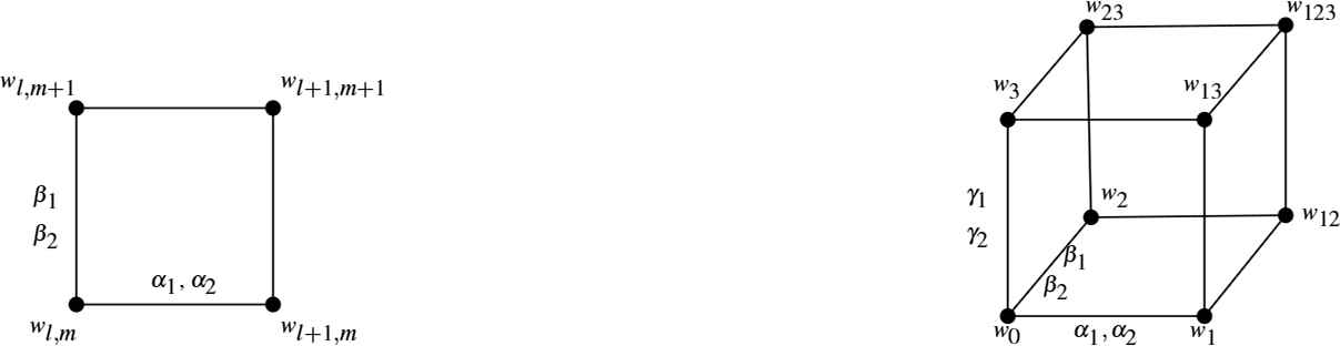
Note that αi and βi, i = 1,2 are parameters, which may also depend on l and m. We assume that the parameters (α1,α2) and (β1,β2) correspond to the l and m directions respectively on the lattice and embed this equation in a cube with a third direction associated with parameters (γ1,γ2), see Figure 3.1 cf. [47].
It is easy to check that if we put the equation with respective associated parameters on each face of the cube and initial values are given at vertices w0,w1,w2,w3, we obtain the same value of w123 from the three possible ways of computing it [3, 24]. This property is called consistency around a cube, or CAC.
The Lax pair of the lattice mKdV equation is well known [24]. In Appendix A, we provide a derivation of the following Lax pair whose compatibility condition, namely M(w1,w12,β1,β2,x)L(w0,w1,α1,α2,x) = L(w2,w12,α1,α2,x)M(w0,w2,β1,β2,x) is the multi-parametric equation (3.1):
where we consider l1 and l2 as constants and x as a spectral variable.
3.1. qPII hierarchy
In this section, suppose n ⩾ 2 is a given, fixed integer. We will derive the qPII hierarchy by using the (n,1)-reduction of equation (3.1) i.e., by imposing wl,m = wl+n,m+1 and taking ui = wl,m where i = l − nm [37, 41].
Figure 3.2 represents this reduction with associated parameters, which are different on each edge. Consider the last edge on the horizontal line in this figure, which joins un to un+1. We assume that the corresponding parameters are given by (qα0,1,qα0,2). This can be seen as a non-autonomous reduction of the general mKdV.
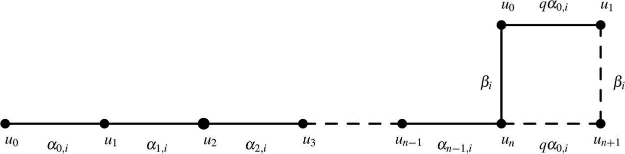
The (n,1)-reduction of mKdV associated with the qPII hierarchy.
On the quadrilateral on the right of Figure 3.2, we have the equation Q(un,un+1, u0,u1; qα0,1,qα0,2,β1,β2) = 0, which is given by
We can solve for un+1 from this equation to find the shift map
Let hj = uj+1/uj for j = 0,1,2 ,...,n− 1, then we obtain the map
We note that the map (3.4) with (3.5) is a general version of the qPII hierarchy given in Theorem 1.1.
Now we will construct the Lax pair for the map (3.4) from the reduction described in Figure 3.2. We start by constructing a monodromy matrix associated with the (n,1)-reduction (see [41]). Walking along the vertices labelled by u0 in Figure 3.2, we have steps taken along horizontal edges, which are represented by L, and one step up in the vertical, which is represented by M, leading to the composition:
This matrix ℒ is called a monodromy matrix.
Applying the deformation
The Lax pair for the quad-equation Q(un,un+1,u0,u1,qα0,1,qα0,2,β1,β2) = 0 is given by
Substitute this in equation (3.7), we get
Thus, we get
Letting A = ℒ and B = L(u0,u1,α0,1,α0,2,x), we obtain a Lax pair of qPII hierarchy.
Taking the parameters as the following
3.2. qPIII hierarchy
First of all, we notice that the deformation operator of
We consider the hierarchy of qPIII starting with (n,1)-reduction, and it can be described by the following Figure:
On the quadrilateral on the right of Figure 3.3, we have the following equations
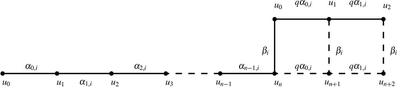
The (n,1)-reduction of mKdV associated with the qPIII hierarchy.
We can solve for un+1 and un+2 from these two equations to find the map
Similar to the hierarchy of qPII, we define
We note that the map (3.11) with (3.12) is the qPIII hierarchy given in Theorem 1.1.
Now as in the qPII hierarchy, we will construct the Lax pair for the map (3.11) from the reduction described in Figure 3.3. Similarly, the monodromy matrix associated with the (n,1)-reduction is given by
Applying the deformation
The Lax pairs for the quad-equations
Using (3.16) and (3.15) in equation (3.14), we get
If we take A = ℒ, B = L(u1,u2,α1,1,α1,2,x)L(u0,u1,α0,1,α0,1,x), we have the Lax pair of qPIII hierarchy.
Remark 3.1
The entries (1,2) and (2,1) of matrix Aj, which we choose to be 1 and − 1 in the matrices, can be replaced with any constants and the compatibility condition still holds.
4. Bäcklund Transformations of the hierarchies
One of the interpretations of CAC property is a connection with Bäcklund transformations. The CAC property can be regarded as a Bäcklund transformation between a top and a bottom equation in a cube [5]. It can be described as follows.
We consider the following quad-equation which is CAC
We then embed this equation (4.1) in the third direction associated with variables v and lattice parameters γ, this parameter will be a Bäcklund transformation parameter (see Figure 3.1 where w3 is replaced with v). A Bäcklund transformation between two equations which are depicted by the top and bottom faces in the cube is given by
We note that this is an auto-Bäcklund transformation as the top and bottom equations are the same.
In this section, we use the Bäcklund transformation of the lattice mKdV to derive the Bäcklund transformation for the qPII and qPIII hierarchies. Moreover, we give a few examples of some rational solutions for second and fourth order.
4.1. Bäcklund transformation of the qPII hierarchy
To find a Bäcklund transformation for the qPII hierarchy, we embed the (n,1) periodic reduction in three dimensions with a slight modification. A third direction in the × × lattice is associated with parameters γ1,γ2 and variables vi’s. Instead of imposing the (n,1) periodic reduction for the v’s variables, we use a twist reduction vl+n,m+1 = vl,m/d cf. [8]. This is because we want to create a Bäcklund transformation between two equations with different parameters. Parameters along the staircase of the v variables are as the same as the ones we use for the u variables. For example the (2,1)- reduction in three dimension corresponding to the first member in the qPII hierarchy can be described in Figure 4.1.
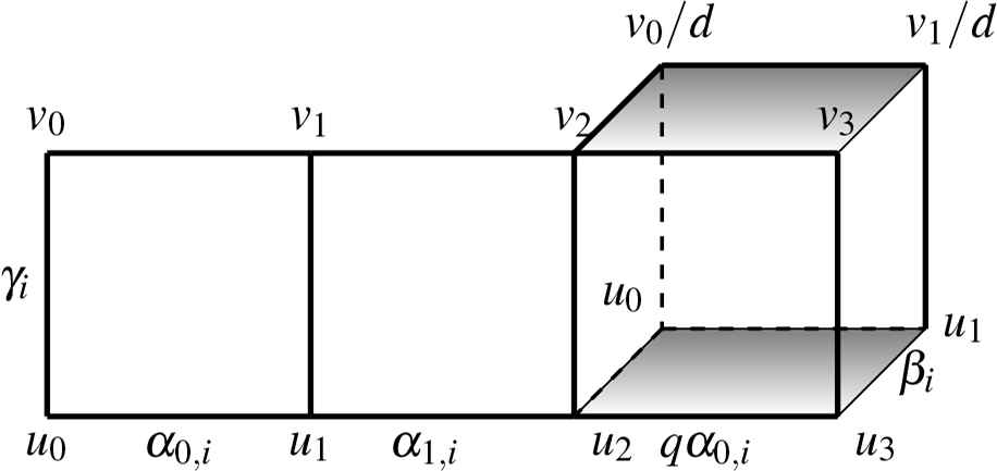
Bäcklund transformation for qPII.
We now illustrate a method of finding a Bäcklund transformation for the qPII hierarchy by using the base case qPII which is associated with n = 2.
The twisted reduction for variables v’s gives the top shaded equation which is given by
This gives us a shift map
As we discussed above, a Bäcklund transformation can be inherited from CAC. Thus, a Bäcklund transformation between the shaded equations in Figure (4.1) is the following system
We consider this system as the system of variables v0,v1,v2. By writing v2 and v1 in terms of v0, we obtain a quadratic equation in v0 which leads to non-rational solutions in general. However, if we take γ2 = 0 then system (4.4) becomes a linear system and it can be solved uniquely with the following solution
This defines the Bäcklund transformation BT : (u0,u1,u2) ↦ (v0,v1,v2). We note that the Bäcklund transformation should be compatible with the shift map Sv and S, i.e. we have
This implies d = q. Similar to the qPII equation, we introduce
This suggests that we introduce Hi = qgi for i = 0, 1, 2, in which case equation (4.5) can be written as
Therefore, H1 satisfies qPII, with parameter λ 2q2 instead of λ 2. Hence, the transformation from hi to Hi, where hi = ui+1/ui, and i = 0,1,2, defines the Bäcklund transformation for qPII. Thus, we can write the Bäcklund transformation of
We can see that this transformation produces a solution, H of qPII with parameter λ2q2 from a solution, h corresponding to λ2.
Proposition 4.1
The simplest rational solution (seed solution) of the qPII and qPIII hierarchies, equations (1.8) and (1.11), respectively is
This can be checked by substituting the above values into (1.8) and (1.11), respectively. Applying the Bäcklund transformation (equation (4.6)) repeatedly on the seed solution will give us an infinite number of solutions of equation (2.1) for λ2↦q2λ2. In the next few examples we will use the notation h(t;λ2) to refer to a solution of equation corresponding to λ2.
Example 4.1
Let us look at few examples of rational solutions of
We note that we can start with another seed solution h1 = − 1 so, we have another infinite solution for
Following the same method above, a Bäcklund transformation for the nth member of the qPII hierarchy (Figure 3.2) is given by the system below
Taking γ2 = 0, we obtain a linear system of v0,v1,...,vn. We also want that this Bäcklund transformation is compatible with the shift map; thus d = q.
Let gi = vi+1/vi, and let the parameters be as given in (3.8). Then, we obtain a Bäcklund transformation of equation (1.8), which is
To obtain the form of
Proposition 4.2
Let hi be a solution of
Corollary 4.1
The Bäcklund transformation of
Example 4.2
We generate the first three rational solutions of the
4.2. Bäcklund transformation of the qPIII hierarchy
We have the qPIII hierarchy given by equation (1.11). We can apply the method given in Subsection 4.1 to the qPIII hierarchy because Figure 3.3 is the same as Figure 3.2 with the square on the right extended one step. Hence, we can deduce the Bäcklund transformation of the qPIII hierarchy.
Proposition 4.3
Let hi be a solution of
This proposition provides us with the following Bäcklund transformation for
Corollary 4.2
The Bäcklund transformation of
Example 4.3
We consider solutions of
In the next Corollary we give the explicit form of Bäcklund transformation for the fourth-order of the qPIII equation.
Corollary 4.3
The Bäcklund transformation of
Example 4.4
Let us give a few solutions of
5. Exact solution of the Lax pairs for q-discrete second and third Painlevé equations
Because the general solutions of discrete Painlevé equations are new transcendental functions, the corresponding solutions of their associated linear problems are highly nontrivial. In this section, we consider special q-rational solutions of the qPII and qPIII equations that exist for special values of parameters and deduce the solutions of their respective linear problems. The results we obtain are similar to those in [20, 31], where rational solutions of qPII and qPIII and their associated linear problem were studied. In the latter paper, the monodromy matrix A was shown to be a product of diagonal matrices and we show that this is also true for the qPII hierarchy as well as the hierarchies of qPIII. The main results of this section are stated in Propositions 5.1 and 5.2.
We use the notation Γq(1 − z) to denote the product
The qPII hierarchy equation (1.8) is solved by (4.7), and this allows its linear system to be diagonalized by a constant matrix. Hence, we can solve it in terms of q-Gamma functions.
Proposition 5.1
Suppose hi are solutions of the qPII hierarchy given by Proposition 4.1. When B and 𝒯 are as given in (1.6) and (1.7), respectively, there exists a solution Φ(x,t) of Lax pair (1.1a,1.1b) given by
Proof
Substituting the special solution (4.7) (take λ = − 1) into the Lax pair (1.1a) and (1.1b), where A is given in (1.3), and B is given in (1.6) gives
We denote the solution matrix of (5.2) and (5.3) as
We now diagonalise both A and B with constant matrix
Let
Equation (5.5a) is solved by writing
These equations (5.7) can be solved in terms of q-Gamma function; therefore we get
Similarly, equation (5.5b) has a solution
Therefore
To find C0(t) and C1(t), we use the deformation problem
This implies
Using (5.8) and (5.9), we obtain
Therefore, we get
Remark 5.1
The simplest solution of the qPII hierarchy given by Proposition 4.1 also happens to be a solution of the qPIII hierarchy under the condition b = 1. Since the qPII and qPIII hierarchies share the same spectral linear problem, it follows that the solution of the linear problem given in Proposition 5.1 is also a solution of the corresponding linear problem for the qPIII hierarchy. The difference is only on the values of parameters bi (i = 0,1,...,n), in the case of qPIII the values take: b0 = b1 = t,
Proposition 5.2
When B and 𝒯 were given in (1.9) and (1.10), respectively, and the qPIII hierarchy equation (1.11) is solved by (4.7), there exists a solution Φ(x,t) of Lax pair (1.1a, 1.1b) given by
6. Conclusion
In this paper, we have presented two hierarchies of Painlevé equations, one of them is a qPII hierarchy which is found in [21] and another is a qPIII hierarchy which is new. Each of these hierarchies was obtained by reduction of the multi-parametric lattice mKdV equation, by using the staircase method. The explicit forms of these hierarchies are given in equations (1.8) and (1.11), with second members of each hierarchy provided by equations (2.8) and (2.10).
In addition to explicit construction of these hierarchies, we provided some properties which are deduced for the first time. One of these is a method to construct Bäcklund transformations for every member of the qPII and qPIII hierarchies. We found so-called seed solutions for each member of these hierarchies. We then used these transformations on seed solutions to find rational solutions of second-order and fourth-order members of the qPII and qPIII hierarchies. From the seed solution for the hierarchies, we also deduced the corresponding solutions of their Lax pair; see Propositions 5.1 and 5.2.
It is noteworthy that the spectral problem in each Lax pair in each hierarchy involves a 2 × 2 coefficient matrix, A from equation (1.1a), which satisfies the conditions of non-resonance in Birkhoff’s theory of linear q-difference equations. To our knowledge, this is the first time such linear problems have been constructed for q-Painlevé hierarchies.
There still remain open questions. In the PDE setting, members of a hierarchy are related by recursion operators. However, such operators are not known in the difference equation setting. We have also not touched upon continuum limits, although there is reason to believe that the hierarchies we have provided have well known Painlevé hierarchies as continuum limits.
Finally, we note that the construction methods in this paper also lead to other hierarchies. These will be the subject of future publications.
A. Derivation of the Lax pair (3.2)
Here we provide how we derive the Lax pair (3.2). Using the CAC property, we obtain a Lax pair of equation (3.1)
Now we replace k1 and k2 in (A.2) and (A.3) with
Acknowledgment
This research is supported by Australian Research Council (ARC) grant FL120100094 and by a grant from the “Research Center of the Female Scientific and Medical Colleges”, Deanship of Scientific Research, King Saud University.
Footnotes
We would like to thank the referee for this observation.
References
Cite this article
TY  - JOUR
AU  - Huda Alrashdi
AU  - Nalini Joshi
AU  - Dinh Thi Tran
PY  - 2020
DA  - 2020/05/04
TI  - Hierarchies of q-discrete Painlevé equations
JO  - Journal of Nonlinear Mathematical Physics
SP  - 453
EP  - 477
VL  - 27
IS  - 3
SN  - 1776-0852
UR  - https://doi.org/10.1080/14029251.2020.1757235
DO  - 10.1080/14029251.2020.1757235
ID  - Alrashdi2020
ER  -