
Evaluating the Effects of Climate and Environmental Factors on Under-5 Children Malaria Spatial Distribution Using Generalized Additive Models (GAMs)
 , Temesgen Zewotir
- DOI
- 10.2991/jegh.k.200814.001How to use a DOI?
- Keywords
- Factor analysis; GAMs; hot-spots; multicollinearity; nonlinear effects; spatial autocorrelation
- Abstract
Although malaria burden has declined globally following scale up of intervention, the disease has remained a leading cause of hospitalization and deaths among children aged under-5 years in Nigeria. Malaria is known to be related to climate and environmental conditions. Previous research has usually studied the effects of these factors, neglecting possible correlation between them, high correlation among variables is a source of multicollinearity that induces overfitting in regression modelling. In this paper, a factor analysis was first introduced to circumvent the issue of multicollinearity and a Generalized Additive Model (GAM) was subsequently explored to identify the important risk factors that might influence the prevalence of childhood malaria in Nigeria. The GAM incorporated the complexity of the survey data, while simultaneously modelling the nonlinear and spatial random effects to allow a more precise identification of the major malaria risk factors that influence the geographical distribution of the disease. From our findings, the three latent factor components (constituted by humidity, precipitation, potential evapotranspiration, and wet days/maximum and minimum temperature/proximity to permanent waters, respectively) were significantly associated with malaria prevalence. Our analysis also detected statistically significant and nonlinear effect of altitude: the risk of malaria increased with lower values but declined sharply with higher values. A significant spatial variability in under-5 malaria prevalence across the survey clusters was also observed; malaria burden was higher in the northern part of Nigeria. Investigating the impact of important risk factors and geographical location on childhood malaria is of high relevance for the sustainable development goals (SDGs) 2015–2030 Agenda on malaria eradication, and we believe that the information obtained from this study and the generated risk maps can be useful to effectively target intervention efforts to high-risk areas based on climate and environmental context.
- Copyright
- © 2020 The Authors. Published by Atlantis Press International B.V.
- Open Access
- This is an open access article distributed under the CC BY-NC 4.0 license (http://creativecommons.org/licenses/by-nc/4.0/).
1. INTRODUCTION
Malaria disease is majorly caused by the protozoan of the Plasmodium types, which comprise the Plasmodium malariae species, the Plasmodium falciparum species, the Plasmodium ovale species and the Plasmodium vivax species, usually transmitted via the infected female Anopheles mosquitoes [1–6]. The global burden of the deadly P. falciparum malaria has declined greatly, but the decline has not been universal, and areas of higher burden persist in many African countries [3]. According to the 2017 World malaria report, the P. falciparum was the most prevalent species of malaria parasite in the African region, which accounted for approximately 99.8% of the estimated severe malaria cases, followed by the South-Eastern Asia 62.8%, the Eastern Mediterranean 69% and the Western Pacific regions 71.9% [3]. From the report, it was also noted that P. vivax was the predominant parasite in the American region. For example, in Venezuela and the Eastern Mediterranean regions, controlling over 70% of all the malaria cases [5–9].
However, among the sub-Saharan African countries, Nigeria has the highest share of the global burden of malaria disease [3]. More than 95% of the malaria cases in Nigeria are caused by P. falciparum [10–12], mostly occurring in children under the age of 5 years [3,10,12]. At present almost more than 70% of the Nigerian population live in endemic areas [13,14]. An important partway to understanding malaria distribution patterns and planning effective intervention strategies is the identification of important influencing factors to malaria prevalence and transmission [8,15].
A challenge in studying malaria risk in Nigeria is the heterogeneity of the prevalence, which is attributed to high variability in climate conditions as well as the landscape [2,16]. Few published studies in Nigeria have linked malaria prevalence to several influencing factors, including climate and environmental conditions [2,10,11,13,15,17–20], socioeconomic factors [15,21–23], geographical factors [10,13–15,18,24], and control strategies as well as prevalence of other febrile illnesses [22,25–27]. Additionally, several authors in other malaria endemic countries have investigated the correlation between malaria and important meteorological variables as observed in Venezuela [6–9], in Zimbabwe [28], in Zambia [29,30], in Côte D’Ivoire [31], in Ghana [32], in Burundi [33], in Ethiopia [34,35] and many more. It was found that malaria infections are not uniformly distributed in space. According to the findings of Grillet et al. [7], Laguna et al. [9], Awolola et al. [17], Nkurunziza et al. [33], the epidemiological patterns of mosquito-borne pathogens could be extraordinarily heterogenous by cause of a complex interactions among parasites, vectors and host, which occurs at definite locations and time, inducing irregular patterns of epidemic spread (malaria), that may reflect spatial variation in the disease distribution.
It is evident that malaria disease is spatially correlated because children living in a given geographical location may exhibit similar behavior that influences the rate of infection. Public health policy makers may want to understand the geographical distribution of malaria across the states and regions rather than just the prevalence across states, and this might shade more light on the distributional patterns across space. In modelling spatial data, the existence of spatial autocorrelation between observations must be considered. Spatial autocorrelation-measure offers additional insight into the interdependence of spatial data and ignoring such correlation can lead to biased and erroneous inference. Progress has been made in understanding the individual risk factors associated with malaria distribution and generally where the burden in higher, but spatial analytical studies on how malaria infection is associated with climate and environmental conditions with respect to under-5 malaria prevalence data are limited in Nigeria. From the literature, we have observed that studies to identify specific clusters of elevated under-5 malaria risks across the states and regions using nationally representative data remains largely unexplored.
This paper evaluates the spatial patterns of under-5 malaria distribution based on the 2015 Nigeria Malaria Indicator Survey (NMIS) data, with the corresponding Demographic and Health Survey (NDHS) geospatial dataset. The main goal was to identify hot-spots of under-5 malaria risks and to investigate important influencing factors with respect to climate and environmental factors, while accounting for the spatial structure of the data. Our study explored a factor analysis to circumvent the issue of multicollinearity among the highly correlated variables by obtaining latent factor component of the observed climate and environmental factors. Subsequently, we used a Generalized Additive Model (GAM) to examine the nonlinear and spatial random effects of the potential malaria risk factors. Other geospatial covariates such as urban-rural settlement, population density, Enhanced Vegetation Index (EVI) and travel times to the nearest population settlement >50,000 inhabitants, were included directly in our analysis, specifically because of the relative lack of literature that explores the impact of the aforementioned factors on under-5 malaria risks in Nigeria. This study may provide information on the geographical patterns of under-5 malaria distribution which could inform public health policy makers and program managers on the priority areas that need enhanced malaria control and intervention across Nigeria.
2. MATERIALS AND METHODS
2.1. Study Area
Nigeria is the largest country in sub-Saharan Africa, a landlocked country of more than 923,768 km2 located in the tropical region within Latitudes 4° and 14° north of the Equator and between Longitudes 2°2′ and 14°30′ east of the Greenwich Meridian [10]. It has 37 regional states, including the Federal Capital Territory (FCT), within the six geopolitical regions (Figure 1). The country shares borders with Niger Republic in the north, the Republic of Chad in the northeast, Republic of Cameroon in the east, and Republic of Benin in the west [12,36]. Nigeria has a tropical climate which is made of two seasons, the wet and dry season, being propelled by the movement of two dominant winds, the rain-bearing southwesterly winds and the cold, dry and dusty northeasterly winds, usually called the Harmattan period. The dry-season lasts for approximately 6 months from October to March, with a spell of coldness accompanied by dry-dusty Harmattan wind, which is felt mostly in the north between December and January. The wet season also last for approximately 6 months from April to September [16,36]. The Nigeria’s temperature oscillates between 25°C and 40°C, with a range of temperature from 2650 mm in the southeast to ≥600 mm in other parts of the north, predominantly on the boundaries of the Sahara desert, while the rainfall ranges from 2650 mm in the southeast to <600 mm in some parts of the north, mainly on the outskirts of the Sahara desert [36]. The country has a wide range of climate and vegetation, the vegetation consists of mangrove swamp forest in the Niger Delta and Shel grassland in the north [37].
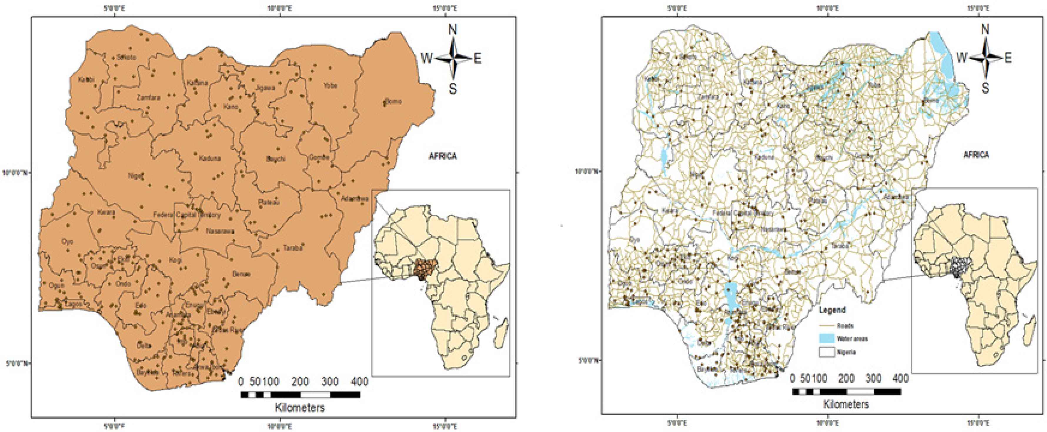
Locations map of where the survey dataset was collected based on the 2015 MIS–DHS in Nigeria’s 37 States, including the Federal Capital Territory (FCT).
2.2. Study Data
This study was based on the available data collected from the NMIS of 2015, with the corresponding NDHS geospatial covariates, assessed upon request from the Measure DHS website (https://dhsprogram.com/data/). The MIS/DHS are internationally reorganized sources of data being designed to generate representative data of key health indicators at national and sub-national (region or state) levels [12,36]. The surveys typically utilized two-stage stratified cluster design in which the country was stratified into the administrative areas and then subsequently stratified into urban and rural areas [12]. At the first stage of sampling, selection of clusters (enumeration areas) from each of the urban and rural strata was involved. At the second stage, households were systematically selected. The selected households were further visited and interviewed by qualified personnel purposely trained for the survey. A detailed review of the sampling methods is presented in the MIS/DHS sampling manual [38]. Three questionnaires including women, household, and the men were carried out in the sampled households. These questionnaires were designed to collect information on the characteristics of households and eligible women, men as well as children. In addition children under the age of 5 years in the selected households, were tested for malaria using Rapid Diagnostic Tests (RDT) to determine the prevalence, with an approved consent from the parents or caregiver [12]. The survey protocol was approved by Nigeria Health Research Ethics Committee of the Federal Ministry of Health.
2.2.1. Outcome variable
In controlling the risk of malaria and reducing the high mortality rate in endemic regions, the World Health Organization recommended timely diagnosis and instant treatment as key strategies, having approved the RDTs for malaria diagnosis in the MIS/DHS surveys [12,39]. In this study, the outcome of interest was based on malaria RDT survey results as a binary indicator of the presence of malaria parasites in the child’s blood sample, where 1 signifies the presence of malaria and 0 the absence. A total number of 6025 observations were included in our analysis.
2.2.2. Explanatory variables
The explanatory variables considered in this study comprise a selection of climate and environmental factors obtained from the DHS Spatial Data Repository upon request (Table 1) [40]. The DHS program georeferenced these climate and environmental data to be used for spatial analysis, by making available standardized files of the most frequently used geospatial covariates (climate and environmental factors) for the year 2015, which can be linked to the MIS datasets via the cluster ID [40]. This study aimed at examining the effects of the selected geospatial covariates (climate and environmental factors) on childhood malaria prevalence in Nigeria. The values of the extracted covariates are based on geographical coordinates of the clusters, therefore, are regarded as cluster level [40]. In addition, the results from a wide range of literature also highlighted the need to include these covariates in malaria analysis, having also been utilized in various spatial modelling and mapping studies in other countries [41–44]. The covariates considered include: the annual precipitation, annual Potential Evapotranspiration (PET), maximum temperature, minimum temperature, cluster altitude, humidity, EVI, wet-days, population density, travel times, proximity to permanent water bodies, and urban–rural settlement. More detailed information on the DHS geospatial data can be found at (http://spatialdata.dhsprogram.com/resources/).
| Covariate | Data sources | Definition |
|---|---|---|
| Enhanced Vegetation Index (EVI) | Nigeria Demographic and Health Survey (NDHS) Spatial Analysis data | The average vegetation index value within the 2 km (urban) or 10 km (rural) buffer surrounding the DHS cluster at the time of measurement (year). The enhanced vegetation index was calculated by measuring the density of green leaves in the near-infrared and visible bands. |
| Proximity to waters (Coast/Large Lakes) | NDHS Spatial Analysis data | Straight-line distance to the nearest major water body. Based on the World Vector Shorelines, CIA World Data Bank II, and Atlas of the Cryosphere. |
| Population density | NDHS Spatial Analysis data | Estimates of human population density is the number of persons/km2 based on counts consistent with national censuses and population registers. |
| Precipitation | NDHS Spatial Analysis data | The average precipitation measured within the 2 km (urban) or 10 km (rural) buffer surrounding the DHS survey cluster each year. |
| Travel time to nearest settlement >50,000 inhabitants | NDHS Spatial Analysis data | The average time (min) required to reach a high-density urban center from the area within the 2 km (urban) or 10 km (rural) buffer surrounding the DHS cluster location, based on year 2015 infrastructure data. |
| Minimum temperature | NDHS Spatial Analysis data | The average annual maximum temperature within the 2 km (urban) or 10 km (rural) buffer surrounding the DHS cluster location. The maximum temperature is calculated from the modeled mean temperature and the modeled diurnal temperature range. |
| Maximum temperature | NDHS Spatial Analysis data | The average annual minimum temperature within the 2 km (urban) or 10 km (rural) buffer surrounding the DHS cluster location. The minimum temperature is calculated from the modeled mean temperature and the modeled diurnal temperature range. |
| Potential Evapotranspiration (PET) | NDHS Spatial Analysis data | The average annual PET within the 2 km (urban) or 10 km (rural) buffer surrounding the DHS cluster location, synthetic measurement that was calculated using a variation of the Penman–Monteith formula. |
| Cluster altitude | NDHS Spatial Analysis | Measure of surface altitude (m). The data were interpolated using a thin plate smoothing spline algorithm with altitude, longitude and latitude as independent variables. |
| Wet days | NDHS Spatial Analysis data | The average number of days receiving rainfall within the 2 km (urban) or 10 km (rural) buffer surrounding the DHS cluster location. It combines the number of observed days with rainfall from weather stations with the number of days that should have received rainfall. |
| Urban–rural settlement | NDHS Spatial Analysis data | This is urban–rural population classification of the area within the 2 km (urban) or 10 km (rural) buffer surrounding the DHS survey cluster location. It is the representation of the degree of urbanization concept obtained using urban-rural settlement classification model adopted by the Global Human Settlement Layer (GHSL) project. |
Climate and environmental covariates, and their definitions
2.3. Variable Selection and Data Analysis
From data explorations, it was observed that the climate and environmental covariates were highly correlated as they reflect related latent characteristics. The high correlation between the variables is a source of multicollinearity in regression models. However, one can circumvent the problem of multicollinearity using factor analysis, because removal of some variables may conceal important information associated with the data [45,46]. In order to identify the potential highly correlated climate and environmental covariates, all the covariate-pairs were compared to the correlation between them using correlation analysis implemented in Statistical Analysis Software (SAS), version 9.4 (SAS Institute Inc., Cary, NC, USA). The pairs with correlations (c > 0.5) as highlighted in Table 2, were further scrutinized [46,47].
| Variables | Precp | Hum | EVI | MaxT | MinT | PET | ProxW | UR | TR | PopD | Alt | WetD |
|---|---|---|---|---|---|---|---|---|---|---|---|---|
| Precp | 1.000 | |||||||||||
| Hum | 0.989* | 1.000 | ||||||||||
| EVI | 0.633* | 0.623* | 1.000 | |||||||||
| MaxT | 0.055 | −0.033 | −0.055 | 1.000 | ||||||||
| MinT | 0.463 | 0.394 | 0.271 | 0.872* | 1.000 | |||||||
| PET | −0.606* | −0.667* | −0.565* | 0.677* | 0.250 | 1.000 | ||||||
| ProxW | −0.616* | −0.633* | −0.518* | 0.310 | −0.099 | 0.791* | 1.000 | |||||
| UR | 0.131 | 0.181 | −0.067 | −0.250 | −0.100 | −0.319 | −0.218 | 1.000 | ||||
| TR | 0.031 | 0.036 | −0.038 | 0.106 | 0.087 | 0.101 | 0.006 | −0.469 | 1.000 | |||
| PopD | −0.145 | −0.085 | −0.307 | −0.452 | −0.392 | −0.270 | −0.092 | 0.601* | −0.310 | 1.000 | ||
| Alt | −0.487 | −0.533* | −0.226 | 0.186 | −0.160 | 0.545* | 0.620* | −0.160 | −0.069 | −0.127 | 1.000 | |
| WetD | 0.957* | 0.959* | 0.686* | 0.070 | 0.499 | −0.629* | 0.624* | 0.184 | −0.002 | −0.109 | −0.443 | 1.000 |
Indicate correlation among variables.
Precp, precipitation; Hum, humidity; EVI, enhanced vegetation index; MaxT, maximum temperature; MinT, minimum temperature; PET, potential evapotranspiration; ProxW, proximity-to-water; UR, urban–rural settlement; TR, travel times; PopD, population density; Alt, cluster altitude; WetD, wet days.
Correlations between the climate and environmental variables (all correlations were significant at 5% level)
In Table 2, we observed a clear pattern of correlation as the results indicated that the following covariates including: the annual precipitation, humidity, PET, maximum temperature, minimum temperature, proximity to permanent water bodies and wet days exhibited high correlation between themselves at 5% level of significance, and the result motivated us to use an additional step using factor analysis to address the issue of multicollinearity associated with highly correlated variables in regression modelling.
Using factor analysis implemented in SAS version 9.4, we transform some of the highly correlated variables into new independent uncorrelated variable known as the latent factors [47]. Rotated factor matrix (i.e. a rotated factor loadings) were obtained as seen in Table 3. The linear combination of these highly correlated climate and environmental factors allowed the identification of three main latent factor components that explained 97% of the total variation of the data. These latent factors included (1) the wet events component which can also be defined as a period of wet season that constituted: the humidity, precipitation, PET, and wet days. (2) The temperature variation, which is a linear combination of the maximum and minimum temperature and (3) proximity to permanent water bodies which formed the third latent factor component. Therefore, subsequent analysis with the GAM, included: the wet events component, the temperature variation, proximity to permanent water bodies and the direct inclusion of other important covariates namely: the EVI, the cluster altitude, urban–rural settlement, population density and travel time to the nearest settlement >50,000 inhabitants (distance to major roads).
| Parameters | Factor 1 (Wet events component) | Factor 2 (Temperature variation) | Factor 3 (Proximity to water bodies) |
|---|---|---|---|
| Annual precipitation | 0.9467* | 0.1313 | −0.2584 |
| Humidity | 0.9567* | 0.0459 | −0.2656 |
| Maximum temperature | −0.0209 | 0.9741* | 0.2151 |
| Minimum temperature | 0.3518 | 0.9244* | −0.0765 |
| Potential evapotranspiration | −0.5819* | 0.5589 | 0.5625 |
| Proximity to permanent water bodies | −0.4099 | 0.1113 | 0.9004* |
| Wet days | 0.9268* | 0.1577 | −0.2978 |
Factors with high loadings.
Results of the estimated Varimax-rotated factor loadings, applying factor analysis for the highly correlated covariates
2.4. Generalized Additive Model
The GAMs are nonparametric regression techniques proposed by Hastie and Tibshirani [48], as an extension to the conventional Generalized Linear Models (GLMs), that allow for nonparametric relationships between a response variable and variety of continuous covariates. The generalized additive models are especially useful, when there are uncertainties about the type of influence of predictors [49]. The model makes use of regression splines in modelling, to provide a flexible way of approximating the underlying regression functions by polynomials and does not assume any specific model for the dependence between covariates and the response variable. Contrary to the GLMs, the GAM tries to fit possible observed data as closely as possible by enabling the smooth effects of the continuous predictors as well as the spatial structure of the data [48–50].
Assume that yi is a binary random variable that indicates whether an under-5 child has malaria parasite, and this is available for 6025 number of children in 37 geographical locations. We assume that the response variable yi whose distribution belongs to the exponential family be associated with covariates of different types including continuous, categorical as well as spatial covariates. Like the GLMs, the mean value µi of the response variable yi is linked to the predictor ηi via the nonlinear link function g(.), such that;
As already stated, the vector of the covariates can be split into fixed covariates xi = (xi1, …, xip)′, continuous covariates (ϑi1, …, ϑiq)′ and spatial covariates in the form of x and y coordinates with plausible nonlinear influence on the predictor ηi. However, unlike the GLMs that assume a linear predictor, the GAMs instead assume a semiparametric additive form for the predictor ηi, by relaxing the linearity assumption in the GLMs using the smoothing terms that characterize the nonlinearity dependency structure [48]. Both the parametric components and unknown nonparametric smooth functions f(.) are accommodated into the GAM, while simultaneously incorporating the spatial effects for the geographical location. The general form of the model with respect to the semiparametric predictor ηi can thus be expressed as:
In this paper, a generalized additive logistic regression model with a logit link function was used to study the under-5 malaria prevalence at the cluster level, and our focus was on the use of this model for the analysis of the continuous variables
This model accounts for the nonlinear effects of the climate and environmental covariates, while simultaneously incorporating the spatial structure of the malaria survey data in terms of geographical coordinates (latitude and longitude). The nonparametric terms were constructed via the penalized regression splines to estimate the nonparametric functions of the model parameters, as well as other covariates involved in the GAM model, while taking account of the spatial autocorrelation [51]. Further, the predicted values from the model was mapped both at state and regional levels to obtain the risk maps of under-5 malaria prevalence. This was done by generating the fitted values; i.e. the values for the malaria RDT outcome predicted by the fitted data via the GAM, on which we utilized the kriging method to infer values in the unsampled locations. This was weighted by the neighborhood distance to the unsampled points, using the weighted combination of the nearby data points [52]. This approach allowed us to model and map the risks of under-5 malaria infections, to identify possible hot-spots of malaria across Nigeria.
The spatial analysis was carried out using ArcGIS, version 10.6.1 (Environmental System Research Institute (ESRI), Redlands, CA, USA) and all the statistical analysis was carried out in SAS statistical software version 9.4. The significance level was set at α = 0.05 and the model diagnostics was performed using the goodness of fit statistics and residual plots [48,49,53].
3. RESULTS
3.1. The Sample Characteristics
This study included 6025 children between ages 6 and 59 months in the analysis. The mean (±SD) age of the children was 4.2 (±1.5) months. Most of the children were males 3079 (50.7%). Regarding their age categories, there were 721 (11.9%) children between ages 6 and 12 months, 1283 (21.1%) between 13 and 24 months, 1309 (21.6%) between 25 and 36 months, 1417 (23.3%) between 37 and 48 months and 1341 (21.1%) between 49 and 59 months, respectively. These children were tested for malaria RDT of which their binary outcome was used as the response variable. Most of these children reside in rural areas 4033 (66.4%) and the percentage of children aged 6–59 months with malaria infection was 2736 (45.1%).
3.2. Association Between Under-5 Malaria Outcome and Climate and Environmental Covariates as Obtained Using Generalized Additive Model
The analysis using a GAM assessed the relationship between malaria prevalence and the climate and environmental covariates, including the latent factors obtained through factor analysis. The findings of these covariates were estimated as nonlinear effects using smoothing splines, results presented in Table 4. Results in Table 4 showed that the degrees of freedom values are much larger than 1 for all the predictors, the measures suggest nonlinear patterns in the dependency of the malaria outcome on the predictors. In addition, the model output revealed that all spline terms are significant in predicting malaria prevalence.
| Covariates | Estimated degree of freedom | F-value | p-value |
|---|---|---|---|
| S (Wet events) | 9.0000 | 27.1206 | 0.0013 |
| S (Temperature variation) | 9.0000 | 19.3509 | 0.0298 |
| S (Proximity to water bodies) | 9.0000 | 43.2202 | <0.0001 |
| S (Cluster altitude) | 8.0000 | 82.5703 | <0.0001 |
| S (Vegetation density) | 7.0000 | 20.5699 | 0.0372 |
| S (Travel time) | 8.0000 | 99.0031 | <0.0001 |
| S (Population density) | 8.0000 | 22.8964 | 0.0035 |
| S (Urban–rural settlement) | 3.0000 | 29.8106 | <0.0001 |
| S (Spatial effects) | 24.4341 | 187.9308 | <0.0001 |
Approximate significance of the smooth terms
Figures 2A–2F, 3A and 3B gives the estimated smoothing components for childhood malaria with their corresponding 95% confidence intervals. The first latent component (constituted by precipitation, humidity, PET, and wet days) was statistically significant and nonlinearly associated with malaria prevalence (p = 0.0013; Figure 2A). The impact of the second latent factor component (constituted by maximum and minimum temperature) was statistically significant: malaria prevalence increased with lower temperature but declined sharply with higher temperature, indicating a negative impact of higher temperature on malaria prevalence (p = 0.0298; Figure 2B). A significant negative nonlinear association was also found for proximity to water bodies (p < 0.0001; Figure 2C), indicating an overall increase in malaria prevalence for shorter distance from water bodies. We observed a decrease in malaria prevalence at increasing altitude (p < 0.0001; Figure 2D), areas below 500 m were found as being at the highest risk of malaria prevalence, whereas areas over 500 m were found as having the lowest risk of malaria. The lowest risk of malaria was observed at altitudes above 500 m. Similarly, vegetation density was found to be significantly and nonlinearly associated with malaria prevalence (p = 0.0372; Figure 2E). The travel times covariate, which measures the amount of time required to reach a settlement of >50,000 people was found to be statistically significant and nonlinear (p < 0.0001; Figure 2F). The pattern of the nonparametric effect showed a wiggly estimate that is hardly interpretable, though the highest risk of malaria was observed at values between 150 and 250 min away. Further, the risk of under-5 malaria prevalence was found to decrease with high population density (p = 0.0035; Figure 3A). In the case of urban–rural settlement, the effect was highly non-monotonic with increasing malaria risks for both low and high values (p < 0.0001; Figure 3B).
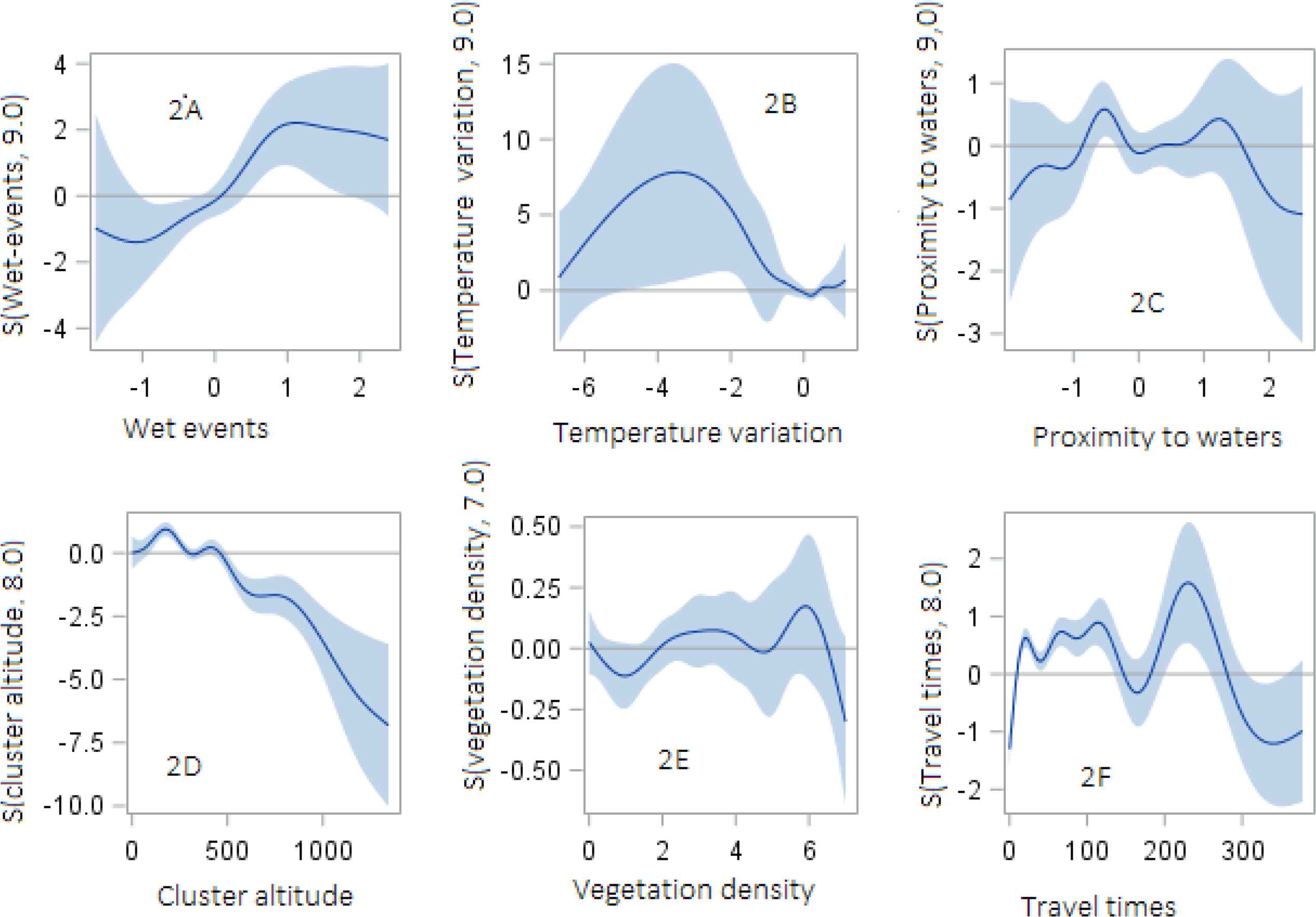
Smoothing plots of relationships between under-5 malaria prevalence and climate-environmental factors in GAM with 95% confidence bands. Panel A: wet events component (precipitation, humidity, potential evapotranspiration, and wet days). Panel B: temperature variation component (maximum and minimum temperature). Panel C: distance to permanent water bodies. Panel D: cluster altitude. Panel E: enhanced vegetation index and panel F: travel times.
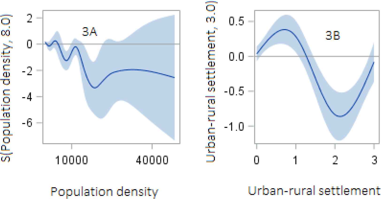
Smoothing plots of relationships between under-5 malaria prevalence and climate and environmental factors with 95% confidence bands. Panel A: population density. Panel B: urban–rural settlement.
3.3. Spatial Variability in Under-5 Malaria Prevalence
This study highlights the spatial variability of childhood malaria prevalence in Nigeria, the non-parametric term which provides information on the spatial variation was statistically significant (p < 0.0001). It was found that the hot-spots of under-5 malaria prevalence were localized predominantly in the North-west, North-east, and partly in the North central regions of Nigeria as seen in Figure 4. Further, the risk map in Figure 5 revealed a highly significant malaria prevalence in the following states: Adamawa, Jigawa, Sokoto and Zamfara states. Other states such as: Benue, Kebbi, Niger, Kwara, Oyo, Kano, and Kastina had slightly higher burden of under-5 malaria as compared to most states in the Southern regions. Malaria risk among children under-5 was found to be significantly very low in the following states: Anambra, Imo, Delta, Abia, Akwa-ibom, Bayelsa, Ogun and Lagos. Notably, the white areas indicate unsampled parts of Borno state in the North east region for the 2015 NMIS, where no malaria observation was obtained, possibly due to security challenges as seen in Figures 4 and 5 [12]. More studies may be required to ascertain the causes of under-5 malaria prevalence in the identified high-risk regions.
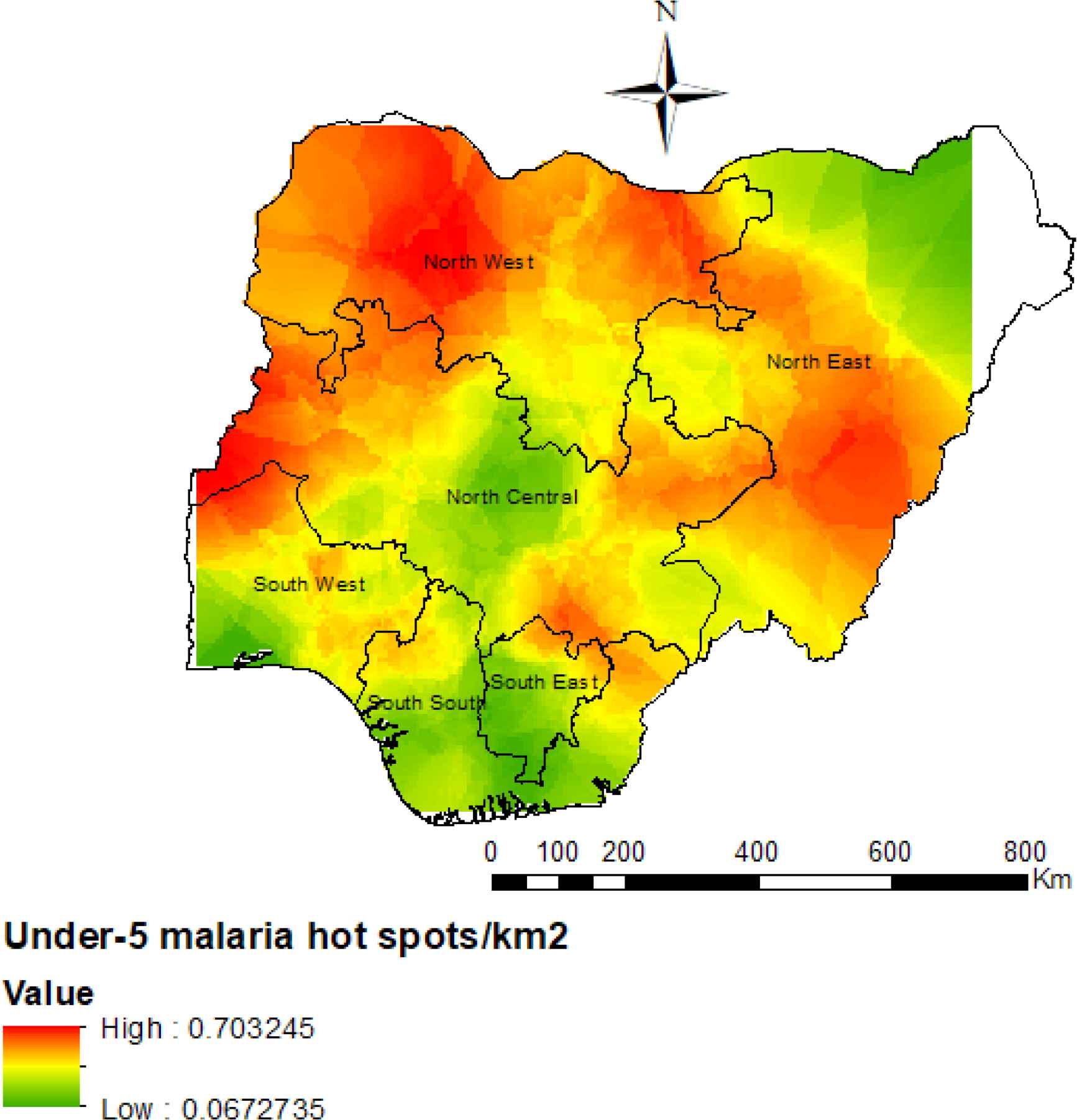
Predicted risk map of malaria prevalence of under-5 children for the six geopolitical regions in Nigeria. Shown is the colorimetric scale representing the risk of malaria per kilometer square.
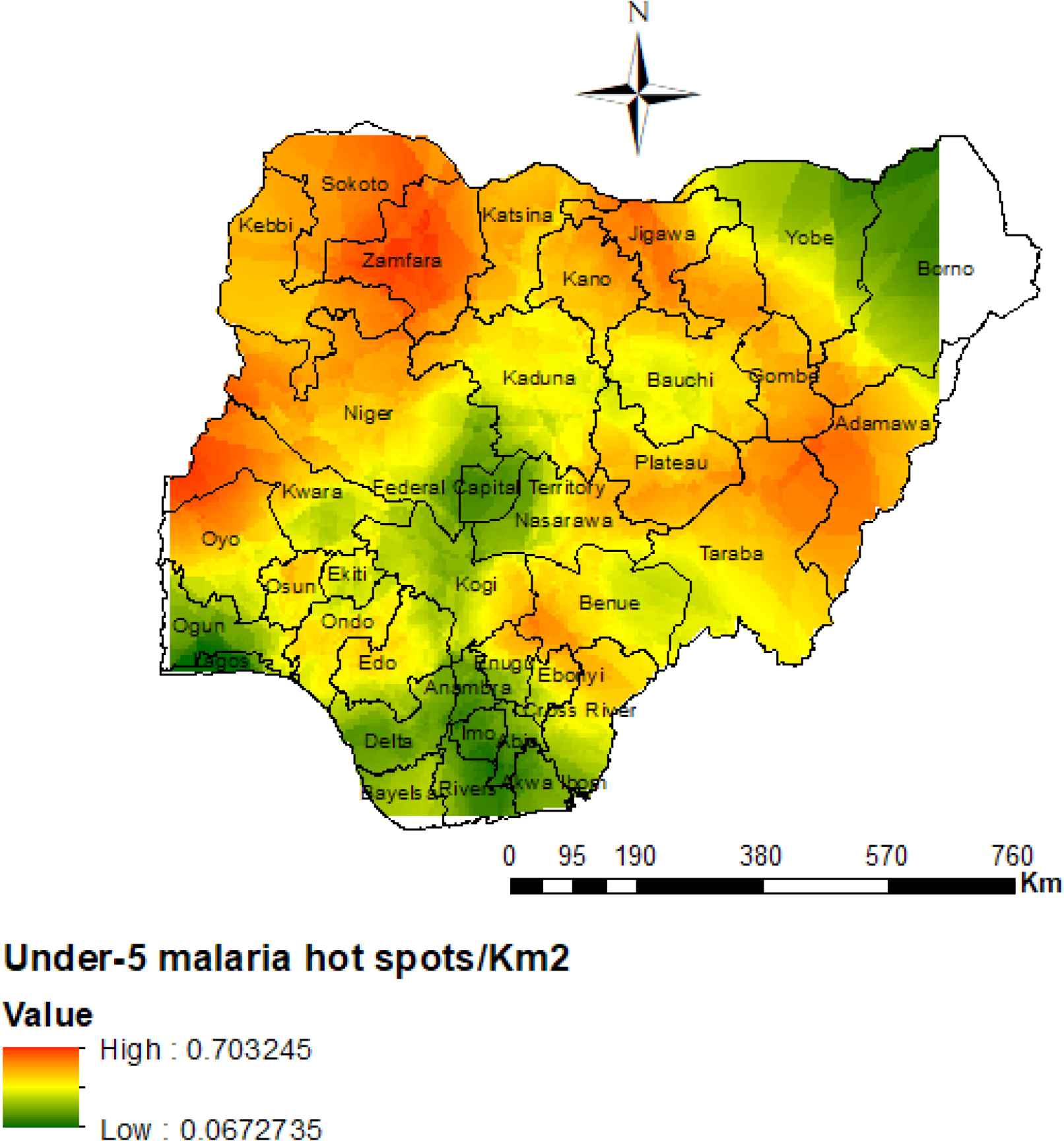
Predicted risk map of malaria prevalence of under-5 children for the 37 states in Nigeria. Shown is the colorimetric scale representing the risk of malaria per kilometer square.
4. DISCUSSION
In this study, a GAM with spline smoothing function and factor analysis were performed to examine the effects of climate and environmental factors on the prevalence of childhood malaria in Nigeria. The factor analysis was used to simplify the complexity of the relationships among the climate and environmental covariates and to improve the effectiveness of predictor variables having transformed the original set of highly correlated variables into a new set of an equal number of latent factors to reduce dimensions and avoid collinearities, whereas the GAM with spline smoothing was performed to capture the nonlinear relationships between malaria prevalence and climate-environmental covariates impacting on its prevalence, including the estimated latent factor components obtained via factor analysis.
The nonlinear relationship between the first latent factor component (constituted by humidity, precipitation, wet days, and PET) and malaria prevalence was similar to that observed elsewhere [29,33,54–56]. Studies have shown that exposed small pools of stagnant water during wet seasons or at the beginning of dry season encourages mosquito survival and larvae development [29,57], as heavy rainfall may flush away the breeding larvae, thereby decreasing the number of malaria causing mosquitoes. The findings of Adigun et al. [15], Nkurunziza et al. [33], Teklehaimanot et al. [35] also indicate a negative impact of strong rains (wet events), which contributes to the destruction of mosquito breeding sites, but an optimal combination of humidity and precipitation supports a good condition for mosquito breeding and development of vectors. However, according to the findings of Shimaponda-Mataa et al. [29], Teklehaimanot et al. [35], Ssempiira et al. [57], the distribution of malaria largely occurs in regions with sufficient precipitation, that provides comfortable mosquito habitats for vector species, where also adequate humidity enables mosquito survival.
The impact of temperature on malaria prevalence has been highlighted in several studies [29,33,35,54,58], indicating a negative effect of maximum temperature. Their findings have identified a positive impact of minimum temperature on malaria transmission, suggesting that mosquito development is usually interrupted at higher temperature, as higher temperatures within a given range could shorten the growth of anopheline mosquitoes, the incubation period as well as viral rate of development. Accordingly, the result of our analysis also showed a positive impact of decreasing temperature as well as a negative impact of increasing temperature on childhood malaria prevalence. The risk of childhood malaria prevalence is observed to decrease with increasing distance from permanent water bodies (rivers, lakes, dams, etc.), indicating a significant nonlinear effect of distance from water bodies on malaria. Water bodies play a very important role as larval breeding sites for malaria occurrence, and the findings of this study has indicated that children residing at a shorter distance from water bodies are found to be at a higher risk of malaria infection. This finding is consistent with the results of Onyiri [13], Adigun et al. [15], Ghebreyesus et al. [34], Ssempiira et al. [57]. According to the literature, closeness of residence to permanent water bodies enhances the risk of malaria, revealing that permanent surface of the waters is an important risk factor for malaria prevalence. Anopheles mosquitoes could breed in sites where water is present for at least 10–15 days or more, whereas permanent water bodies creates mosquito breeding sites that may possibly aid malaria transmission all year round.
A significant negative nonlinear association was found between population density and the risk of malaria infection, contrary to the findings of Nkurunziza et al. [33], Samadoulougou et al. [59]. Logically, areas with high population density are usually urban where access to health facilities and better environmental conditions are higher; this might reduce possible exposure to malaria infection among under-5 children. Urbanization leads to decrease in malaria through reduction in human-vector contact and vector breeding sites [60]. According to the literature, urbanization has been historically linked to development [61]. Urban populations, excluding those residing in slums normally have better access to healthcare and better quality of life for children, and generally more economically prosperous than the rural dwellers, thus, resulting in an improved living conditions, and a higher likelihood of affording better health care and treatment, which reduces the risk of childhood malaria and associated deaths. Result of Figure 3B which captured the nonlinear effect of urban–rural differences in malaria prevalence was highly non-monotonic, implying that the risk of malaria infection is high amongst inhabitants dwelling in both rural and possibly urban slums, meaning that children residing with both rural and urban households, possibly those children living in urban slums are highly vulnerable to malaria infection. Inhabitants residing in rural and slummy areas are generally poor, and usually face problems including access to public health resources and poor environmental sanitation. Therefore, adequate intervention and general child’s living conditions are expected to significantly reduce the proportion of malaria prevalence in such populations.
Furthermore, the relationship between under-5 malaria prevalence and cluster altitude were found to be nonlinear and statistically significant. Malaria infection decreased monotonically with increasing altitude; the result indicated a decreasing malaria probability at increasing altitude. From the results, areas below 500 m were found as being at the highest risk of malaria prevalence, whereas areas over 500 m were found as having the lowest risk of malaria exposure. This may be logical since, most of the malaria infections usually occur in coastal areas where altitude is lower, the nonlinearity effect showed a sharp decrease in malaria risk as altitude increased, similar to the findings of Onyiri [13], Adigun et al. [15], Gunda et al. [29], Chirombo et al. [62]. Findings also indicated that altitude may indirectly influence the distribution and spread of malaria through its effect on temperature, being that at certain altitudes malaria transmission does not occur due to high temperature, which does not favor the life cycle of the parasite. The EVI was also nonlinear and significantly associated with malaria prevalence, malaria risk was significantly higher for high vegetation index value. The EVI is an important factor that indicates a condition suitable for agricultural production (which enhances the spread of malaria) [63]. According to several authors [64,65], vegetation indices such as EVI are considered proxies of vector habitat; disease transmission and physical environment are strongly correlated with disease environments in determining the intensity of a child’s exposure to infectious diseases such as malaria. The case of clearing vegetation during farming season by farmers may also unintentionally lead to creation of mosquito breeding sites [64,66].
Findings on the travel times covariate, which measures the amount of time required to reach a settlement of >50,000 people, being also defined as areas near the major roads was found to be statistically significant with an extreme wiggly estimate that is hardly interpretable, though we observed a risk of contracting malaria peak at a distance between 150 and 250 min away, and this is of a particular interest. The result is not surprising, because travel times was computed to provide a useful composite measure of the extent to which areas are being connected to the national system of transportation [40]. For instance, areas near major roads, would generally be well connected, even if they were some distance away from the major cities, thus having higher access to population centers, public health scare resources as well as quality health care systems [67]. Similar studies have also indicated that distance and travel time to population centers in some sub-Saharan African countries are highly correlated with wealth and developmental indices, implying that a population’s social and health welfare decreases rapidly as entry or access to population centers gets worse [68,69]. Therefore, the effectiveness of any public health intervention measure against childhood malaria can also be determined by the distance from a residence in which a child lives to the major roads.
This study highlighted the spatial variability of childhood malaria prevalence across all the states and regions of Nigeria. Despite increasing efforts in fighting the disease, malaria prevalence among the under-5 children remain high. There is evidence of significant clustering of childhood malaria, with higher malaria risk occurring in the northern states, more especially in Adamawa, Sokoto and Zamfara states, but lower in the southern regions. Although the risk varied substantially across states and regions in Nigeria, and such variability may be associated with the underlying climate and environmental conditions. These spatial patterns may also indicate possible unobserved risk factors of malaria, which may be state- or region-specific or that which transcends geographical boundaries of the states and regions under consideration. Public health interventions should therefore be targeted in the high-risk areas to reduce the malaria prevalence and to achieve effective malaria control. Further epidemiological research may be required for more clarification using additional information at different spatial scales within the study areas.
The limitation of this study is that, the study used a cross-sectional data from the NMIS, the nature of the secondary data did not allow any causal relationship to be established. In addition, there are many other influencing factors that were not included in our analysis, which may bias the results. However, the strength of this research lies in the ability to generalize the findings to the whole country, having utilized nationally representative survey data of internationally good quality and being able to quantify the state- and regional-level variations in childhood malaria prevalence in Nigeria based on climate and environmental context. With more robust statistical models, this study may be extended to incorporate several other influential factors that were not considered in this present study.
5. CONCLUSION
The main goal of our study was to evaluate important risk factors of under-5 malaria prevalence with respect to climate and environmental conditions using a GAM, the methodology that has shown a greater level of flexibility than the standard regression models. Studying the spatial variations in under-5 malaria prevalence in a country like Nigeria is an effort in the right direction as it could help discover areas where malaria control and intervention should be enhanced. The Nigerian government need to consider the identification of remote cause of high malaria prevalence considering the effect of climate change. It was evident from our results that Nigeria’s climatic conditions make it suitable for high malaria transmission all year round. Therefore, being able to identify important climate and environmental conditions that are conducive to the under-5 malaria prevalence will help to predict when malaria transmission may likely occur and how to effectively target the disease control and prevention across the identified high-risk areas in Nigeria.
CONFLICTS OF INTEREST
The authors declare they have no conflicts of interest.
AUTHORS’ CONTRIBUTION
CLJU obtained permission to use the 2015 NMIS/geospatial data sets. CLJU and TZ conceptualized the modeling idea and CLJU performed the analysis. Both CLJU and TZ jointly drafted and revised the manuscript. The manuscript is part of CLJU’s PhD work. All authors read and approved the final manuscript for submission.
FUNDING
No financial support was provided.
ACKNOWLEDGMENTS
This work is part of the first author’s Ph.D. thesis under the supervision of the second author at the University of KwaZulu-Natal, South Africa. The authors would like to thank the Measure DHS for the permission granted to use the NMIS and NDHS-GPS data in this research. The first author appreciates the study leave and the opportunity granted by the University of Nigeria Nsukka, Nigeria. The first author thanks the Department of Biostatistics, University of Washington, United States, for the training and the opportunity given to her during the 10th Annual Summer Institute in Statistics and Modeling in Infectious Diseases (SISMID).
ABBREVIATIONS
- GAMs,
generalized additive models;
- DHS,
Demographic and Health Surveys;
- MIS,
Malaria Indicator Survey.
Footnotes
Data availability statement: The data utilized in this study are freely available and the access was granted before use. The raw data may be accessed upon request, through Measure Demographic Health Survey (DHS) websites: www.dhsprogram.com/data/ and Data Repository ( http://spatialdata.dhsprogram.com ).
REFERENCES
Cite this article
TY  - JOUR
AU  - Chigozie Louisa Jane Ugwu
AU  - Temesgen Zewotir
PY  - 2020
DA  - 2020/08/21
TI  - Evaluating the Effects of Climate and Environmental Factors on Under-5 Children Malaria Spatial Distribution Using Generalized Additive Models (GAMs)
JO  - Journal of Epidemiology and Global Health
SP  - 304
EP  - 314
VL  - 10
IS  - 4
SN  - 2210-6014
UR  - https://doi.org/10.2991/jegh.k.200814.001
DO  - 10.2991/jegh.k.200814.001
ID  - Ugwu2020
ER  -