
Estimating the Effect of AfCFTA on Intra-African Trade using Augmented GE-PPML
- DOI
- 10.2991/jat.k.211122.001How to use a DOI?
- Keywords
- AfCFTA; GEPPML; International trade agreements; CGE; MRT; RTA
- Abstract
This paper draws on a general equilibrium poisson pseudo maximum likelihood model augmented by a dynamic capital accumulation to estimate the effects of the African Continental Free Trade Agreement (AfCFTA) on intra-African trade flows. The empirical results show that the AfCFTA could raise intra-African trade by 24% in the short term and slightly more in the long run. However, the potential trade and welfare gains associated with the continental trade integration reform are expected to vary across countries, with the largest gains accruing to countries that exhibit relatively low intra-regional trade performance and level of integration pre-AfCFTA.
- Copyright
- © 2021 African Export-Import Bank. Publishing services by Atlantis Press International B.V.
- Open Access
- This is an open access article distributed under the CC BY-NC 4.0 license (http://creativecommons.org/licenses/by-nc/4.0/).
1. INTRODUCTION
Regional integration has played a key role in the economic development and diversification of exports in other regions of the world. In particular, supporting the growth of cross-border investment and the development of regional value chains has played a catalytic role in the structural transformation of European and Asian economies. Over time, it has deepened the process of economic integration and sustained the growth of intra-regional trade. The African Continental Free Trade Agreement (AfCFTA), which entered into force earlier this year, has been touted as a game-changer. It has the potential to transform African economies and diversify the sources of growth and exports in a region where the expansion of cross-border trade has been undermined by the supply-side constraints as well as tariff and Non-Tariff Barriers (NTB) (Green et al., 2019; Fofack, 2020). This paper aims to ex-ante estimate the potential impact of the AfCFTA on intra-African trade flows.
Previous studies on African Regional Trade Agreements (RTAs) either had the objective of ex-post estimating the effects of existing RTAs or ex-ante evaluating prospective Free Trade Agreements (FTAs). Earlier ex-post studies had mixed findings on the success of RTAs in promoting intra-African trade (Afesorgbor, 2017). However, recent studies provide more robust and coherent results. In particular, several Regional Economic Communities (RECs), including Economic Community of West African States (ECOWAS), Common Market for Eastern and Southern Africa (COMESA), Southern African Development Community (SADC), and to a lesser extent, East African Community (EAC), seem to have a positive and significant effect on bilateral trade between their members. At the same time, other RTAs are less successful (e.g., MacPhee and Sattayanuwat, 2014; Afesorgbor, 2017; Candau et al., 2019). Ex-ante studies, on the other hand, give moderately optimistic predictions on the outcomes of AfCFTA. These studies generally use Computable General Equilibrium (CGEs) models to simulate the decrease in tariffs or the removal of quotas associated with the establishment of a larger RTA (Mevel and Karingi, 2012; Sandrey and Jensen, 2015; Mold and Mukwaya, 2016; Saygili et al., 2018; Abrego et al., 2019; Green et al., 2019; Maliszewska et al., 2020).
This article draws on the General Equilibrium Poisson Pseudo Maximum Likelihood (GEPPML) method to predict the potential effects of the AfCFTA on intra-African trade flows (Anderson et al., 2015a).1 This method uses the properties of structural gravity and PPML to compare various consequences of a counterfactual policy scenario against a baseline scenario. The static procedure is composed of three stages; first, we estimate the elasticity of bilateral trade to trade costs (in this case, joining an RTA) and use it to estimate trade costs for each trading pair. Second, we estimate the hypothetical trade costs associated with forming a continental free trade area (AfCFTA) and use them to estimate counterfactual trade flows. Then, we evaluate the change in bilateral trade flows due to AfCFTA while considering the change in Multilateral Resistance Terms (MRTs), maintaining expenditure and output values constant. The third stage relaxes the constant income and expenditure assumptions. It employs the estimates from the first and second stages to evaluate the full endowment general equilibrium repercussions on trade and welfare, given fixed factor endowments. In the dynamic stage, we introduce capital accumulation to the model, following Anderson et al. (2015b), to study the evolution of trade over time.
To the best of our knowledge, Anderson et al. (2015b) and Anderson et al. (2015a) are the only studies employing the proposed methodology, while Candau et al. (2019) is the only study that uses GEPPML on African data. They evaluated the welfare effects of existing African RTAs. The proposed methodology has several interesting features. In contrast to CGEs, it does not impose strong assumptions on the functional form of the relationship between different aggregates or the value of the parameters. In addition, it is less data-intensive and will be more suitable in the African context, where the dearth of time series data has been a significant constraint to econometric analysis and, specifically, the application of CGE. Instead, it uses the properties of PPML to capture the observed and unobserved variables with country-time and pair-specific fixed effects and maintains an extremely strong level of goodness-of-fit. GEPPML thus benefits from the extensive research and debate on the best econometric approach to estimate the relationship between trade costs and bilateral trade. Simultaneously, it quantifies the effect of policy intervention, an absent feature in ex-post econometric studies. However, as a tool for policy experiments, GEPPML yields similar results to CGEs and Exact-hat Algebra when specified correctly (Bekkers, 2019).
Our findings show that forming an AfCFTA would increase intra-African trade by about 24.07% compared to the baseline in a static setting. It would further increase to reach 25.26% in the long run when we introduce dynamic capital accumulation, with the average effect of forming an RTA on bilateral trade set at 120.1%. The general equilibrium feedback is expected to be small because there is a positive counterweight to the negative tendencies of MRTs following the implementation of the AfCFTA and given the small size of African economies relative to the rest of the world.
This paper is organized as follows: Section 2 discusses the analytical framework and reviews the channels through which RTAs can affect intra-African trade. Section 3 describes the empirical methodology of the paper. Section 4 discusses the results and Section 5 concludes.
2. THEORETICAL FRAMEWORK
The GEPPML procedure is an empirical application to the gravity model, arguably the standard framework for analyzing trade policy. Gravity models started with an atheoretical observation of trade flows. Trade between two countries is proportional to the product of their Gross domestic product (GDP) and inversely proportional to the distance between them. Subsequent studies laid the theoretical foundations for such observation, inspired by the Ricardian, Armington (Constant Elasticity of Substitution; CES), and Heckscher-Ohlin frameworks (Head and Mayer, 2014). Although structural gravity is mainly concerned with trade, it is flexible enough to allow growth models to be incorporated into it to study the effect of trade liberalization on a wide range of economic indicators, such as welfare and investment.
We follow the framework developed by Anderson et al. (2015b). Underpinning that framework is the introduction of a dynamically endogenous production and capital accumulation to the standard static structural gravity model conceived by Anderson and van Wincoop (2003). In this framework, consumers in each country choose between multiple products differentiated by place of origin to maximize their utility under a certain budget constraint, with a defined production function and law of motion for capital. The maximization problem yields Equations (1)–(6). According to Yotov et al. (2016) topology, FTAs affect trade and growth through four layers. The first two layers, partial effect [Equation (1)] and conditional general equilibrium [Equations (1)–(3)], are trade channels, while the latter two, full endowment general equilibrium [Equations (1)–(4)] and dynamic general equilibrium [Equations (1)–(6)], are growth channels.
Xij,t is country i’s exports to country j in year t, and Yi,t, Ej,t and Yw,t are exporter total output, importer total expenditure, and world output, respectively. The exporter’s output reflects its capacity to produce and export, whereas the importer’s expenditure represents a fraction of its income and capacity to buy. The variable tij,t is the trade costs between the pair; it includes natural barriers such as distance and contiguity, and policy variables such as tariffs and regulations. Pj,t and πi,t are the inward and outward MRTs; the former represents the relative barriers to the importer’s world imports, and the latter is the relative barriers to the exporter’s world exports. pi,t represents the factory gate prices, αi is an exogenous CES preference parameter, τ is a discount factor, and φi,t is the trade balance equal to the ratio of expenditure to production. The constant returns to scale Cobb–Douglas production function in Equation (5) has the output as a function of Ai,t, representing technology, Li,t as labor supply and Ki,t as the capital stock, with Ki,0 being given. The rate of capital depreciation is set as δ and the output elasticity to factors as η.
The complexity of the network of existing RTAs in Africa provides a rich area of analysis within this framework when studying the trade effects of the AfCFTA. This is because, within the AfCFTA, African countries are partners in new FTAs with other African countries. Simultaneously, they are considered third parties to FTAs signed by other African countries. To the extent that partner and third-party effects generally go opposite ways, the general equilibrium feedback to the AfCFTA in all layers has an undetermined direction depending on country size and its prior degree of integration in the existing RTA networks.
2.1. Trade Channels
The first layer of the system of equations above explains the current level of bilateral trade between African countries and the direct partial effect of trade liberalization on intra-African trade. The relatively low level of intra-African trade is the consequence of, first, the generally poor condition of infrastructure, non-tariff measures (Odjo et al., 2019), and the vast size of the continent, rendering trade costs high. Second, the deficit of diversification and excessive dependency on primary commodities in a region where manufactured goods dominate cross-border trade has been another major constraint (UNCTAD, 2019). In partial equilibrium, the AfCFTA is supposed to increase bilateral trade between African countries. Considering Equation (1), a decrease in bilateral trade costs associated with signing an RTA will increase trade flows between the pair; the elasticity of substitution between varieties (σ) is larger than 1 by construction.
In conditional general equilibrium, a change in trade costs impacts countries’ terms of trade with others through the MRTs, assuming fixed output and expenditure values. All else held constant, higher MRTs mean that the pair face higher trade barriers and difficulty accessing the world market and the world accessing theirs; they would thus tend to trade more with each other. Another interpretation is that every importer assigns a share of its expenditure and every exporter a share of its production to each country in the world, as a function of trade costs and weighted prices faced by importers and exporters, i.e., MRTs (Head and Mayer, 2014).
When partners sign an FTA, their MRTs decrease, meaning that, on average, market access to both countries improves, thus weakening the direct effect of the FTA on bilateral trade between them. The MRT counterweight is stronger when the partner country is larger, but it is never strong enough to change the direction of the effect (Yotov et al., 2016). For non-member countries, their MRTs increase since they become more isolated relative to member countries, thus increasing trade flows between them. The effect of an RTA on the MRTs of member and non-member countries is stronger when partner countries are larger.
The AfCFTA is modeled as a network of FTAs because African countries are signatories and third parties at the same time. This implies that the conditional general equilibrium feedback can go either way, depending on whether a country is a member of a larger RTA and its size. Let us consider a case of a small African country X, a member of a large RTA, COMESA, for instance. On joining the AfCFTA, X signs an FTA with a small number of countries compared to another country, Z, that is not well integrated into the continent (a North African country). The direction of change in MRTs is undetermined. First, X’s MRTs should decrease due to the signing of new FTAs, and this feedback is stronger the smaller X is. On the other hand, X’s MRTs will also increase since Z signs an FTA with many other countries, restricting X’s market access. The conditional general equilibrium feedback can thus potentially amplify the effect of joining the AfCFTA since the formation of the AfCFTA could increase a member’s MRTs.
2.2. Growth Channels
The third layer of this framework, the full endowment general equilibrium, allows the factory gate prices to respond to trade costs and MRTs changes. Thus, the fixed output and expenditure value assumptions in the first two layers are relaxed while maintaining productive capacity—endowment—constant. Trade liberalization within this layer affects bilateral trade mainly through its effect on country size. As shown in Equation (4), there is a negative relationship between factory gate prices and Outward MRTs (OMRTs), implying that signatories will see their factory gate prices increase, analogous to an increase in demand. The price change will translate into higher export and output values. Since bilateral trade is a positive function of country size, the full endowment feedback goes against and possibly outweighs the conditional general equilibrium effect, and increases bilateral trade between member countries.
For third parties, factory gate prices decrease, and the same mechanism works mostly the opposite way. Because production and expenditure are denominators in the MRTs equations, and since the country size effect can possibly outweigh the price effect, the full endowment general equilibrium feedback can positively affect bilateral trade between a liberalizing country and a third party (Yotov et al., 2016). Within the AfCFTA, the full endowment feedback on African countries will be determined by the direction of change in OMRTs in conditional general equilibrium. They will be treated as partners if MRTs decrease and as third parties if they increase. If the MRTs had positive tendencies, the full endowment effect on trade would be lower than the conditional effect.
Up to this point, we analyzed the effect of the AfCFTA in a static setting, with endowment assumed to be constant and the adjustment happening as consumers and producers adjust their behavior with price changes. The fourth layer introduces a dynamic element to the system. Here, capital accumulation, thus real production, is endogenous and determined within the model. In Anderson et al. (2015b), labor endowment and technological change are exogenous, and the effect of trade policy propagates in time through investment. The change in trade costs positively affects investment in partner countries through the change in factory gate prices and Inward MRTs (IMRTs).
First, higher factory gate prices increase the marginal product of capital, thus encouraging producers to invest. Second, since IMRTs are a price index for imported capital goods, these being cheaper, investments will increase. Third, IMRTs are also a price index for imported consumption goods, rendering them cheaper and leaving more room for saving (Yotov et al., 2016). Higher investment and production further increase bilateral trade between partner countries, compared to the static setting. In other words, the change in trade costs will trigger a deviation from an initial equilibrium to a new steady-state, with static welfare gains amplified by a dynamic path multiplier [Anderson et al. (2015b)]. This is why the effect of AfCFTA on intra-African trade could be higher in a dynamic setting relative to the static model.
3. EMPIRICAL FRAMEWORK
This section employs GEPPML to quantify the effects of the AfCFTA in partial, conditional, full endowment (Anderson et al., 2015a) and dynamic general equilibrium (Anderson et al., 2015b). The policy intervention in our case is the expansion of existing African RTAs into a continent-wide free trade agreement. The static phase—i.e., from the start to full endowment—consists of three stages; the first step is to derive an estimate of the partial effect of RTAs (or any policy variable affecting trade costs). The second stage uses the first stage results to estimate a baseline (pre-policy intervention) and counterfactual trade flows while accounting for the conditional general equilibrium feedback. The third stage uses the estimates of the previous stages to compute the change in factory gate prices. It employs them to evaluate the full endowment general equilibrium effects on welfare and trade (similar to Candau et al., 2019, for the case of African RTAs. For dynamic general equilibrium, we add a fourth stage to quantify the long run effects of trade liberalization through its impact on investment.2
3.1. First Stage
The first stage of the GEPPML derives a consistent estimator for the average effect of RTAs on bilateral trade flows. The issue of how to best estimate the gravity equation is a rich area of research in the economic literature. Even with its high explanatory power, it still suffers from potential problems that could be critical in a trade policy context. As Anderson et al. (2015a) pointed out, it is unnecessary to use PPML in the first stage; instead, any econometric approach that provides an adequate estimate of the partial effect can be used in the second stage.3 We thus provide our estimate for the first stage coefficients, tackling the issues facing the estimation of structural gravity models in the literature. The first issue is the prevalence of zero observations in trade matrices. Second, an atheoretical representation of the gravity equation is likely to yield biased estimators due to the omission of relevant variables and the negligence of key mechanisms correlated with the error term, such as MRTs and self-selection into RTAs.
Trade matrices generally contain many zero observations; log-transforming the dependent variable and using Ordinary Least Squares (OLS) entails a loss of zero observations. This method is problematic because the zeroes are not distributed randomly; there are economic reasons for why some pairs do not trade with each other, and they are likely correlated with the right-hand side variable in question. Different methods such as Tobit to deal with truncation and the Heckman selection model to deal with selection bias were proposed as solutions. However, they were criticized for their vulnerability to heteroskedasticity and the difficulty in finding adequate instrumental variables satisfying the exclusion restriction, respectively (Kareem and Kareem, 2014).
Silva and Tenreyro (2006) suggested using the PPML method to estimate the gravity equation. This method is popular in the gravity literature because of its suitable properties. As a non-linear method, it does not require taking the log of the dependent variable and provides consistent estimates in the presence of heteroskedasticity. Moreover, it solves the adding up problem; the predicted trade flow in the PPML model is exactly equal to the effective flows. Other methods systematically overestimate trade flows (Arvis and Shepherd, 2013), an issue when estimating trade flows following a policy intervention (Fally, 2015). We thus refrain from log-linearizing the gravity equation, and we formulate the model as Equation (7).
We add μi,t and θj,t as importer-time and exporter-time fixed effects, respectively, to account for MRTs and other importer- and exporter-specific observable and unobservable determinants of bilateral trade.4 Capturing MRTs in this formula is crucial to take into consideration the conditional general equilibrium feedback. They are correlated with the independent variable, which is likely to bias the estimates if not included in the model (Anderson and van Wincoop, 2003). There are different methods to solve the omitted variable bias from neglecting the MRTs in the regressors, such as estimating the variable using non-linear programming, using a remoteness index, and introducing country-time fixed effects. We adopt the latter since the first solution is computationally intensive and the second lacks theoretical justification (Head and Mayer, 2014). Fally (2015) demonstrated the exact equivalence between the exporter- and importer-time fixed effects and the MRT in the PPML model. Therefore, using the exporter-time and importer-time fixed-effects is the best solution due to its relative simplicity and theoretical soundness.
We also include γi,j, a symmetric pair fixed effect.5 It has become a common practice in structural gravity models to include a pair fixed effect to take into account time-invariant unobservable trade frictions between the pair (Baier and Bergstrand, 2007; Baier et al., 2019). Countries tend to self-select into RTAs, for countries with prior strong commercial ties tend to form RTAs (Magee, 2003; Egger et al., 2011). Baier and Bergstrand (2007) suggested that there could be barriers to trade that are positively correlated with the probability of forming an RTA (for example, a large anticipated welfare gain) and negatively correlated with bilateral trade flows. Biasness stems from unobserved policies, regulations, or barriers within the partners’ borders that cannot be captured by the standard gravity variables or institutional and political indicators.
3.2. Second Stage
For the second stage, we use the average RTA effect from the first stage
We set our counterfactual scenario as a continental FTA represented by a dummy variable RTAc taking the value of 1 for all African pairs except for internal trade and zero otherwise. This setting enables us to answer the following question: What would the trade flows between African countries have been if they had formed a CFTA in the baseline period? GEPPML is usually implemented to quantify the effects of existing RTAs by setting the counterfactual scenario as if they did not exist, not by simulating an expansion of an RTA (as in Yotov et al., 2016; Anderson et al., 2015a; Candau et al., 2019). Anderson et al. (2015a) and Kumar and Shepherd (2019) are exceptions, as the former simulated the implementation of the Transatlantic Trade and Investment Partnership, and the latter the Trade Facilitation Agreement.
We estimate the counterfactual trade flows using PPML constrained by the counterfactual trade costs
Following the properties of PPML in Fally (2015) and Anderson et al. (2015a), we can quantify the OMRT and IMRT for both the baseline and counterfactual scenarios in Equations (10) and (11).8 We assume the elasticity of substitution σ = 4.8.
3.3. Third Stage
Building on the first two stages, we endogenize the value of output and expenditure by allowing factory gate prices to change as in Equation (4). We solve Equations (1)–(4) to obtain the full endowment MRTs, trade, expenditure, and output, with prices adjusting to satisfy
3.4. Fourth Stage
The fourth stage introduces endogenous capital accumulation to GPML. It is performed by solving Equations (1)–(6). We solved the equation in changes instead of levels, as shown in Anderson et al. (2015b), who followed the approach of Dekle et al. (2007 and 2008). The mechanism shown in the previous subsection is augmented by the change in capital accumulation in Equations (14) and (15), which is obtained by dividing Kj,t+1 by Kj,t in Equation (6). The change in IMRTs and factory gate prices generated by the AfCFTA will induce a change in the capital stock, thus country size, which affects trade then MRTs, prices and so on. This process is repeated until we reach a new steady-state satisfying Equation (16).
The advantage of this method is that it only requires data on trade flows and abstracts some of the parameter assumptions in its level counterpart. It is not necessary to provide an estimate for initial capital stocks, technology or labor endowments. Instead, Kj,0 is set to be 1, and for each country, the trade policy effect is channeled through the capital stock deviating from 1. It is possible to estimate the parameters η and δ within the system, but we opt to use values within the interval of the estimates of Anderson et al. (2015b). We will have η = 0.6 and δ = 0.053.9
4. THE EFFECT OF AfCFTA ON TRADE AND WELFARE
4.1. Data
We use a bilateral trade matrix of 119 countries spanning from 1988 to 2012. We supplemented the country list in Anderson et al. (2015b)10 with missing African countries, increasing the number of African countries to 51.11 Data on bilateral trade are extracted from the TRADHIST dataset (Fouquin and Hugot, 2016). We used the Head and Meyer (2014) dataset for dyadic gravity variables (language, contiguity and distance). We constructed the data on major African RTAs12 using their various respective websites and the WTO. However, we include other FTAs (e.g., Egypt-Ghana FTA) present in the CEPII dataset and Mario Larch’s Regional Trade Agreements Database from Egger and Larch (2008).13 For trade flows, we use 3-year intervals to allow for trade to adjust to changes in trade costs.14 We include intra-national trade flows, defined as apparent consumption (the difference between total production and exports). Since data are not readily available in most African countries, especially after 2006, we approximate production by nominal GDP.15
4.2. Results
Table A2 shows the results of the regression in Equation (6). The first column decomposes the FTA effect into the major RTAs in Africa and other FTAs. Column (2) shows the effect of each RTA and (3) the average effect of a compilation of all intra-African FTAs and non-African FTAs. Column (1) shows that major RTAs in Africa had a positive and significant average effect of e0.789 − 1 = 120.1% on bilateral trade flows. However, the value of the coefficient is primarily driven by the positive effect of COMESA, SADC, and ECOWAS shown in column (2). These results are relatively similar to the coefficients reported in Afesorgbor (2017) and Candau et al. (2019), two recent studies on African RTAs with comparable methodologies.
There is strong evidence that the characteristics of trading pairs and trade agreements determine whether and how successful RTAs are in promoting trade between its members (Vicard, 2011; Cheong et al., 2015; Baeir et al., 2019). We would expect the effect of a new FTA on bilateral trade flows to vary according to the characteristics of the pair and the RTA to which they belong. But for the sake of simplicity, we use the average effect of RTAs (the coefficient in the first column) in the second stage to simulate the expansion into the AfCFTA. This coefficient (
The effect of the AfCFTA on aggregate African trade in different stages is reported in Table 1. In the static model, the exercise yields a 25.2% increase of intra-African trade flows in conditional general equilibrium and 24.07% in full endowment general equilibrium compared to the baseline. Similarly, the share of intra-African trade in total African exports is expected to increase from 11.9% in the baseline17 to 14.6% in conditional general equilibrium and slightly decreases to 14.55%. Accounting for the full endowment feedback is marginal, with the share of intra-African trade in total African exports remaining stable at 14.55%. The discrepancy between the second and third stages is because in many African countries, OMRTs increase, thus reducing the factory gate prices, which in turn cause negative feedback on output and expenditure values, thus full endowment trade levels. However, in the long run, since capital accumulation depends on both OMRTs and IMRTs, and since the combined sign of the change in these variables is negative, the country size effect will dominate, and trade will recuperate its positive tendency. The dynamic model yields a 25.26% increase in intra-African trade compared to 24.07% in the short run.
| Conditional GE (%) | Full endowment GE (%) | Dynamic GE (%) | |
|---|---|---|---|
| Intra-African trade | 25.20 | 24.07 | 25.26 |
| Share of intra-African trade. Baseline = 11.9% | 14.60 | 14.55 | 14.59 |
| Total African exports | 2.42 | 1.85 | 2.60 |
| Total African imports | 2.77 | 2.39 | 2.72 |
| African exports to the ROW | −0.67 | −1.17 | −0.48 |
| African imports from the ROW | −0.77 | −1.04 | −0.85 |
| African real output growth (welfare) | – | 0.119 | 0.294 |
GE, general equilibrium; ROW, rest of the world.
The effect of AfCFTA on African trade and growth (percentage change from the baseline)
Although a 120.1% increase in bilateral trade seems significant in proportional terms, in sheer volume, the change is small due to the weak initial levels of bilateral intra-African trade. AfCFTA will stimulate trade in all African countries (Table A3); total African exports are expected to increase by 1.85% and imports by 2.39% in the static model and will increase to 2.6% and 2.72% in the dynamic model. As for trade with the rest of the world, in the short term, the AfCFTA could divert trade away to African countries, but in the long run, the level of trade with the rest of the world will recover and approach its pre-AfCFTA levels (Table 1).
The long-term effects of the AfCFTA on intra-African trade seem modest at first glance, but this is not entirely the case. When we look at the dynamic welfare gains of AfCFTA, we find that the dynamic path multiplier, i.e., the dynamic welfare gains divided by the static welfare gains, takes the value of 2.47 at a continental level. This number is significantly higher than the estimate found in Anderson et al. (2015b), where the dynamic path multiplier from North American Free Trade Agreement (NAFTA)18 was about 1.6.
However, in contrast to North America, the initial value and share of intra-African trade are relatively low, and the base effect may largely drive the higher value of the dynamic path multiplier. This translates into an overall low impact on capital accumulation and thus the relatively small welfare gains in the short- and long term; 0.119% in the static model and 0.294% in the dynamic model (Tables 1 and A4, and Figure A1). The scope of dynamic results is small because the size of African countries is small compared with the rest of the world, and the level of intra-African trade is relatively low initially. This implies that, while the change in trade in the first step is large, the general equilibrium feedback is low.19
In addition, since the dynamic gains depend on the general equilibrium feedback, these gains are low because the feedback, through MRTs, from the AfCFTA is low. There are two explanations to this observation: first, the position of each country in the agreement as signatories and third parties simultaneously; second, due to the small size of African economies relative to the world economy. To the extent that the value of intra-African trade is initially low, even a large percentage change will yield quantitatively low changes. Furthermore, we observe in Tables A4 and A5 that OMRTs or IMRTs increase in many countries. This implies that the negative tendency from each country signing an RTA does not always outweigh the positive tendencies of MRTs due to the increased remoteness of each country when surrounding countries sign an RTA.
In other words, an increase of OMRTs suggests that the AfCFTA could raise the competition African exports face, even within Africa. For similar reasons, IMRTs increases in some cases, reflecting that exporters, including African exporters, face fiercer competition within several individual African markets. The scope of the dynamic effects reflects the weak general equilibrium feedback. At the same time and to the extent that net change in MRTs is negative in most African countries, investment, thus output and trade, increased over time in the dynamic model, as shown in Table A4 and Figure A1.
The change in intra-African trade flows is driven by the signing of new bilateral FTAs and, to a lesser extent, the general equilibrium feedback. If we ignore the feedback, the AfCFTA will only create trade between a pair with no prior FTA, at least in the short run. Given that Africa has already reached a high level of regional integration, many countries will realistically sign a new trade agreement with only a handful of other countries under AfCFTA. This is why we observe a wide disparity in the trade creation effect, as shown in Table A3. In full endowment general equilibrium, the change in exports to Africa varies between −3.14% in Tanzania and 157.65% in São Tomé and Principe. Smaller Southern African countries (Botswana, Lesotho, Eswatini, etc.) are concentrated at the bottom of the gain distribution; most of them are already part of two large and successful RTAs (COMESA and SADC) and seem to sustain major negative general equilibrium feedbacks. North and Central African countries are concentrated at the top because the former possess a weak level of integration with other African countries, and the RTA of the latter is ineffective. In the long run, the difference between both groups will be sustained.
4.3. Comparison with Past CGE Studies
As predicted by Bekkers (2019), our results are situated within the interval of predictions in past CGE studies, especially those that simulate a reduction in tariff measures. These studies estimate the change in intra-African trade following AfCFTA to be between 4.3% and 32.8%, with a range varying between 24% and 25.3%. The gains in intra-African trade derived from our study are at the higher end of the spectrum. Furthermore, these studies predict the welfare gain to vary between 0.037% and 0.97%, while our estimates were anywhere between 0.119% and 0.294%.20
We can count three studies that used a Global Trade Analysis Project (GTAP) dataset based model (Table 2). First, Sandrey and Jensen (2015), when a number of African “willing” countries eliminate tariffs on intra-African trade, they predicted a 0.70% welfare gain. Saygili et al. (2018) predicted a 32.8% increase in intra-African trade in the long run when all tariffs are eliminated under AfCFTA and a 24.2% increase when some products are exempted. They also found a 2.5% increase in total exports and a 0.97% increase in welfare gain if all tariffs were eliminated. A more recent study by Maliszewska et al. (2020) predicts a 21.76% increase in intra-African trade and 0.13% welfare gain if all tariffs were gradually removed. Other studies found comparable results; for instance, Green’s (2019) study yielded a 16% increase when 90% of tariffs on taxed intra-regional trade flows were removed. The African Development Bank (AfDB) (2019) predicted a 0.1% welfare gain and 14.6 growth in intra-African trade if all tariffs within the area were removed. Abrego et al. (2019), under different specifications—perfect competition and monopolistic competition—concluded a welfare gain between 0.037% and 0.053%.
| Study | Policy | Span | Intra-African trade (%) | Exports (%) | Imports (%) | GDP growth (%) |
|---|---|---|---|---|---|---|
| This study | Removal of some tariff and NTBs based on existing RTAs | Short-run | 24.07 | 1.85 | 2.39 | 0.12 |
| Long-run | 25.26 | 2.60 | 2.72 | 0.29 | ||
| Maliszewska et al. (2020) | Gradual removal of 97% of tariffs on intra-AfCFTA trade | – | 21.76 | 1.78 | 2.31 | 0.13 |
| Gradual removal of 97% of tariffs on intra-AfCFTA trade and some NTBs | – | 51.85 | 18.84 | 19.58 | 2.24 | |
| Gradual removal of 97% of tariffs on intra-AfCFTA trade; 50% reduction in NTBs; implementation of TFA | – | 92.07 | 28.64 | 40.61 | 4.20 | |
| Saygili et al. (2018) | Removal of all tariffs on intra-AfCFTA trade | Long-run | 32.8 | 2.5 | 1.8 | 1.0 |
| Green et al. (2019) | Removal of 90% of tariffs on taxed intraregional trade flows | – | 16.0 | – | – | – |
This table is based on Maliszewska et al. (2020).
TFA, trade facilitation agreement.
Findings in some CGE literature
Studies that went further or modeled a reduction in NTBs showed a more pronounced growth in intra-African trade and welfare. Mevel and Karingi (2012) simulated a customs union following AfCFTA. They estimated the increase in intra-African trade to be 52.3% and the share of intra-African trade to grow from 10.2% to 15.5% within a decade of implementation of the AfCFTA. If some or all NTBs were removed, the welfare gain from intra-African trade could be between 1.25% and 2.24%, and intra-African trade could increase by 51.85% (Maliszewska et al., 2020) and could reach 107.2%, according to AfDB (2019).
Our results are consistent with those obtained under a reduction in tariffs reflects the nature of past African RTAs. Our first stage coefficient generally captures the tariff and NTB reduction associated with the RTAs. However, it is apparent that these realistically affected only tariff barriers, which is evident by the low tariffs applied within RTAs and the high NTBs still in place (Odjo et al., 2019). This is why our simulation, using the first stage coefficient, points to a decrease in tariffs rather than an overhaul of existing trade barriers.
5. CONCLUSION
This paper had the objective of evaluating the intra-African trade prospects of the AfCFTA. We used an augmented GEPPML model to simulate a free trade area encompassing all African countries in conditional, full endowment and dynamic general equilibrium. We found that the formation of an AfCFTA is associated with a 24.07% increase in intra-African trade in the short run and 25.26% in the long run. The effect of the AfCFTA is expected to vary greatly depending on the prior degree of integration of each partner and their sizes. Countries that are not part of any major RTAs or non-performing RTAs are expected to gain the most from the AfCFTA. However, the general equilibrium feedback on trade is low and could reduce the dynamic path multiplier effect on intra-African trade in the long run.
This paper sheds the light on the importance of including countries not presently integrated into any of the major African RTAs in the AfCFTA to simulate intra-African trade. These countries will benefit the most from the agreement in terms of welfare gain and trade. It also provides some optimistic insights into the potential offsetting feedback and diversion effects of signing an FTA that are of utmost concern to policymakers; they are nearly insignificant. In addition, all African countries are expected to have a positive net welfare gain and capital accumulation, even if trade creation is low, sometimes negative, in a few countries. Lastly, compared with other studies, this paper shows the importance of taking the measures in past African RTAs further; giving equal importance to tariff and NTBs, as the latter constitutes the majority of intra-African trade costs.
The only source of endogenous growth considered in this paper was capital accumulation, which is a simplistic assumption. The AfCFTA could further promote African development and trade through human capital accumulation and technological progress critical for industrialization and the expansion of intra-African trade. The flexibility of the proposed framework allows such extension. On the other hand, it will be valuable to study the effect of AfCFTA on the nature of trade; whether it increases the diversity of flows or is skewed towards a certain sector. Structural gravity is malleable enough to allow the usage of GEPPML to perform a sectoral analysis of the AfCFTA, to evaluate the different aspects of AfCFTA (tariffs, quotas, exemptions, etc.) and to study the contribution of country characteristics (infrastructure, geography, etc.). These are important areas for future research that could be investigated to galvanize more support for the implementation of the AfCFTA.
CONFLICTS OF INTEREST
The authors declare they have no conflicts of interest.
AUTHORS’ CONTRIBUTION
HF, RD and OAMH conceived and contributed to the development of the analytical framework. OAMH carried out the data collection and computations. All authors contributed to the analysis of the results and to the writing of the manuscript. HF supervised the research project.
FUNDING
No financial support was provided.
ACKNOWLEDGMENTS
The authors would like to thank Augustin Fosu and the anonymous reviewers for their helpful comments and constructive suggestions on an earlier version of this paper.
APPENDIX
| Country list | |||
|---|---|---|---|
| Algeria | Denmark | Lebanon | São Tomé and Principe |
| Angola | Djibouti | Lesotho | Saudi Arabia |
| Argentina | Dominican Republic | Liberia | Senegal |
| Australia | Ecuador | Libya | Seychelles |
| Austria | Egypt | Lithuania | Sierra Leone |
| Azerbaijan | Equatorial Guinea | Madagascar | Singapore |
| Bangladesh | Eswatini | Malawi | Slovakia |
| Belarus | Ethiopia | Malaysia | South Africa |
| Belgium | Finland | Mali | Spain |
| Benin | France | Mauritania | Sri Lanka |
| Botswana | Gabon | Mauritius | Sudan |
| Brazil | Gambia | Mexico | Sweden |
| Bulgaria | Germany | Morocco | Switzerland |
| Burkina Faso | Ghana | Mozambique | Thailand |
| Burundi | Greece | Namibia | Togo |
| Cabo Verde | Guatemala | Netherlands | Tunisia |
| Cameroon | Guinea | New Zealand | Turkey |
| Canada | Guinea-Bissau | Niger | Turkmenistan |
| Central African Republic | Hungary | Nigeria | Tanzania |
| Chad | India | Norway | Uganda |
| Chile | Indonesia | Oman | Ukraine |
| China | Iran | Pakistan | United Arab Emirates |
| China, Hong Kong SAR | Iraq | Peru | United Kingdom |
| Colombia | Ireland | Philippines | United States |
| Comoros | Israel | Poland | Uzbekistan |
| Congo | Italy | Portugal | Venezuela |
| Côte d’Ivoire | Japan | Qatar | Viet Nam |
| Croatia | Kazakhstan | Republic of Korea | Zambia |
| Czech Republic | Kenya | Russian Federation | Zimbabwe |
| D.R. of the Congo | Kuwait | Rwanda | |
Country list
| Exports | (1) | (2) | (3) |
|---|---|---|---|
| RTA | 0.789*** (0.192) | – | – |
| CEMAC | – | −0.0650 (0.387) | – |
| COMESA | – | 0.698* (0.368) | – |
| ECOWAS | – | 0.489** (0.242) | – |
| EAC | – | 0.192 (0.147) | – |
| WAEMU | – | 0.170 (0.195) | – |
| SADC | – | 0.884*** (0.226) | – |
| Other African FTAs | 0.343 (0.215) | 0.191 (0.239) | – |
| Non-African FTAs | 0.299*** (0.0866) | 0.299*** (0.0866) | – |
| All FTAs | – | – | 0.300*** (0.0864) |
| Pair FE | Yes | Yes | Yes |
| Exporter-time FE | Yes | Yes | Yes |
| Importer-time FE | Yes | Yes | Yes |
| Observations | 106,956 | 106,956 | 106,956 |
| R-squared | 0.9999 | 0.9999 | 0.9999 |
Robust standard errors in parentheses (clustered by pair).
p < 0.1,
p < 0.05,
p< 0.01.
First stage results
| Total exports | Exports to Africa | |||||
|---|---|---|---|---|---|---|
| Conditional (%) | Full (%) | Dynamic (%) | Conditional (%) | Full (%) | Dynamic (%) | |
| Algeria | 1.72 | 1.07 | 1.83 | 60.78 | 58.24 | 60.66 |
| Angola | 0.54 | −0.05 | 0.62 | 22.43 | 21.49 | 22.47 |
| Benin | 3.51 | 4.14 | 3.52 | 12.90 | 12.19 | 12.60 |
| Botswana | 0.46 | 0.60 | 0.58 | 1.06 | 1.54 | 1.24 |
| Burkina Faso | 8.14 | 9.87 | 8.09 | 15.57 | 16.26 | 15.27 |
| Burundi | 4.71 | 5.62 | 4.51 | 7.26 | 6.59 | 6.71 |
| Cabo Verde | 4.31 | 5.69 | 4.31 | 43.89 | 43.33 | 43.36 |
| Cameroon | 11.45 | 12.07 | 11.96 | 65.21 | 66.10 | 65.91 |
| Central African Republic | 19.15 | 19.83 | 19.54 | 78.14 | 77.87 | 78.43 |
| Chad | 2.16 | −0.12 | 2.27 | 52.20 | 47.51 | 52.05 |
| Comoros | 1.90 | 1.78 | 1.84 | 7.28 | 5.69 | 6.90 |
| Congo | 1.39 | −0.28 | 1.79 | 82.99 | 78.61 | 83.37 |
| Côte d’Ivoire | 5.00 | 4.64 | 5.52 | 14.90 | 13.75 | 15.27 |
| D.R. of the Congo | 3.26 | 3.37 | 3.35 | 8.50 | 8.17 | 8.48 |
| Djibouti | 4.79 | 5.59 | 4.70 | 10.62 | 9.93 | 10.19 |
| Egypt | 2.40 | 2.73 | 2.44 | 26.00 | 25.32 | 25.79 |
| Equatorial Guinea | 1.64 | −0.75 | 1.95 | 86.20 | 80.07 | 86.42 |
| Eswatini | 0.72 | 0.70 | 0.76 | 1.32 | 1.31 | 1.35 |
| Ethiopia | 4.04 | 5.04 | 3.96 | 11.47 | 10.82 | 11.00 |
| Gabon | 2.82 | 0.24 | 3.28 | 83.06 | 77.02 | 83.55 |
| Gambia | 6.62 | 7.93 | 6.64 | 19.36 | 18.14 | 18.80 |
| Ghana | 6.19 | 7.91 | 6.40 | 26.33 | 28.34 | 26.54 |
| Guinea | 4.85 | 5.55 | 5.04 | 31.75 | 31.28 | 31.67 |
| Guinea-Bissau | 2.19 | 1.59 | 2.16 | 6.90 | 4.08 | 6.40 |
| Kenya | 7.19 | 9.28 | 7.24 | 14.62 | 15.34 | 14.34 |
| Lesotho | 0.82 | 0.83 | 0.90 | 2.71 | 3.17 | 2.87 |
| Liberia | 3.68 | 4.09 | 4.69 | 65.54 | 65.55 | 66.96 |
| Libya | 0.83 | −0.31 | 0.98 | 29.27 | 26.64 | 29.25 |
| Madagascar | 5.90 | 7.19 | 6.13 | 45.90 | 47.86 | 46.23 |
| Malawi | 0.91 | 0.84 | 0.96 | 2.01 | 1.97 | 2.06 |
| Mali | 10.50 | 12.97 | 10.40 | 18.73 | 19.75 | 18.28 |
| Mauritania | 6.42 | 5.39 | 7.21 | 47.30 | 44.28 | 48.09 |
| Mauritius | 0.68 | 0.63 | 0.72 | 5.64 | 5.00 | 5.53 |
| Morocco | 5.88 | 6.75 | 6.13 | 76.22 | 76.81 | 76.41 |
| Mozambique | 0.42 | 0.50 | 0.47 | 1.62 | 2.11 | 1.74 |
| Namibia | 3.05 | 3.53 | 3.18 | 8.63 | 9.54 | 8.82 |
| Niger | 4.72 | 5.41 | 4.79 | 14.89 | 15.06 | 14.83 |
| Nigeria | 1.81 | 0.89 | 1.91 | 31.78 | 29.71 | 31.69 |
| Rwanda | 6.70 | 8.84 | 6.35 | 7.77 | 8.33 | 7.08 |
| São Tomé and Principe | 20.32 | 28.77 | 20.78 | 140.12 | 157.65 | 141.08 |
| Senegal | 8.71 | 10.90 | 8.74 | 18.92 | 19.73 | 18.59 |
| Seychelles | 0.88 | 0.76 | 0.96 | 6.13 | 5.47 | 6.09 |
| Sierra Leone | 8.97 | 10.42 | 9.35 | 49.06 | 50.33 | 49.45 |
| South Africa | 3.25 | 2.55 | 3.48 | 23.79 | 22.42 | 23.92 |
| Sudan | 0.79 | 0.78 | 0.78 | 6.12 | 4.99 | 5.84 |
| Tanzania | 0.16 | −0.23 | −0.01 | −0.70 | −3.14 | −1.32 |
| Togo | 5.79 | 5.42 | 6.28 | 13.69 | 12.16 | 13.95 |
| Tunisia | 6.36 | 6.89 | 6.93 | 66.99 | 67.65 | 67.81 |
| Uganda | 6.68 | 8.56 | 6.43 | 9.17 | 9.07 | 8.48 |
| Zambia | 0.22 | 0.30 | 0.21 | 0.30 | 0.34 | 0.27 |
| Zimbabwe | 0.34 | 0.58 | 0.39 | 0.64 | 1.09 | 0.72 |
Trade effects of AfCFTA
| Full | Dynamic | Full | Dynamic | ||||
|---|---|---|---|---|---|---|---|
| Output (%) | Output (%) | Capital accumulation (%) | Output (%) | Output (%) | Capital accumulation (%) | ||
| Algeria | 0.057 | 0.211 | 0.210 | Liberia | 1.301 | 1.708 | 1.668 |
| Angola | 0.050 | 0.189 | 0.138 | Libya | 0.003 | 0.297 | 0.278 |
| Benin | 0.085 | 0.147 | 0.140 | Madagascar | 0.229 | 0.379 | 0.370 |
| Botswana | 0.169 | 0.216 | 0.054 | Malawi | 0.044 | 0.105 | 0.088 |
| Burkina Faso | 0.118 | 0.200 | 0.191 | Mali | 0.183 | 0.272 | 0.220 |
| Burundi | 0.154 | 0.198 | 0.115 | Mauritania | 0.671 | 1.375 | 1.346 |
| Cabo Verde | 0.078 | 0.096 | 0.050 | Mauritius | 0.041 | 0.094 | 0.093 |
| Cameroon | 0.392 | 0.792 | 0.782 | Morocco | 0.237 | 0.424 | 0.421 |
| Central African Republic | 0.512 | 0.886 | 0.692 | Mozambique | 0.023 | 0.047 | 0.030 |
| Chad | −0.004 | 0.264 | 0.229 | Namibia | 0.478 | 0.551 | 0.146 |
| Comoros | 0.261 | 0.298 | 0.064 | Niger | 0.111 | 0.205 | 0.197 |
| Congo | 0.138 | 0.700 | 0.687 | Nigeria | 0.030 | 0.186 | 0.183 |
| Côte d’Ivoire | 0.507 | 0.987 | 0.982 | Rwanda | 0.116 | 0.152 | 0.121 |
| D.R. of the Congo | 0.134 | 0.258 | 0.236 | São Tomé and Principe | 1.464 | 1.638 | 0.627 |
| Djibouti | 0.400 | 0.454 | 0.126 | Senegal | 0.220 | 0.350 | 0.338 |
| Egypt | 0.046 | 0.088 | 0.087 | Seychelles | 0.254 | 0.344 | 0.165 |
| Equatorial Guinea | 0.114 | 0.691 | 0.543 | Sierra Leone | 0.468 | 0.739 | 0.622 |
| Eswatini | 0.189 | 0.250 | 0.089 | South Africa | 0.251 | 0.516 | 0.425 |
| Ethiopia | 0.048 | 0.070 | 0.056 | Sudan | 0.024 | 0.042 | 0.035 |
| Gabon | 0.101 | 0.787 | 0.775 | Tanzania | 0.002 | 0.008 | 0.005 |
| Gambia | 0.283 | 0.410 | 0.314 | Togo | 0.561 | 1.069 | 1.057 |
| Ghana | 0.215 | 0.339 | 0.327 | Tunisia | 0.517 | 0.913 | 0.908 |
| Guinea | 0.211 | 0.369 | 0.358 | Uganda | 0.127 | 0.187 | 0.183 |
| Guinea-Bissau | 0.544 | 0.683 | 0.231 | Zambia | 0.009 | 0.026 | 0.026 |
| Kenya | 0.233 | 0.350 | 0.343 | Zimbabwe | 0.016 | 0.037 | 0.037 |
| Lesotho | 0.459 | 0.502 | 0.054 | ||||
Real output and capital accumulation effects of AfCFTA
| Outward multilateral resistance | Inward multilateral resistance | Factory gate prices | ||||||
|---|---|---|---|---|---|---|---|---|
| Conditional (%) | Full (%) | Dynamic (%) | Conditional (%) | Full (%) | Dynamic (%) | Full (%) | Dynamic (%) | |
| Algeria | −0.21 | −0.45 | −0.25 | 0.12 | 0.30 | 0.09 | 0.36 | 0.17 |
| Angola | −0.19 | −0.57 | −0.37 | 0.14 | 0.29 | 0.06 | 0.34 | 0.17 |
| Benin | 0.34 | 0.73 | 0.43 | −0.39 | −0.66 | −0.42 | −0.58 | −0.36 |
| Botswana | −0.09 | −2.30 | −2.19 | 0.09 | 0.01 | −0.10 | 0.18 | 0.08 |
| Burkina Faso | 0.84 | 1.84 | 1.06 | −0.90 | −1.55 | −0.94 | −1.43 | −0.86 |
| Burundi | 0.73 | 1.60 | 0.92 | −0.77 | −1.41 | −0.87 | −1.26 | −0.75 |
| Cabo Verde | 0.51 | 1.13 | 0.65 | −0.53 | −0.96 | −0.58 | −0.88 | −0.52 |
| Cameroon | 0.20 | 0.43 | 0.28 | −0.52 | −0.73 | −0.64 | −0.34 | −0.32 |
| Central African Republic | 0.36 | 0.72 | 0.42 | −0.63 | −1.11 | −0.93 | −0.60 | −0.46 |
| Chad | −0.74 | −1.74 | −1.03 | 0.66 | 1.32 | 0.58 | 1.31 | 0.71 |
| Comoros | 0.11 | 0.18 | 0.09 | −0.13 | −0.45 | −0.38 | −0.19 | −0.12 |
| Congo | −0.56 | −1.26 | −0.70 | 0.25 | 0.85 | 0.17 | 0.99 | 0.46 |
| Côte d’Ivoire | 0.01 | 0.03 | 0.06 | −0.44 | −0.53 | −0.56 | −0.02 | −0.17 |
| D.R. of the Congo | 0.12 | 0.25 | 0.15 | −0.22 | −0.34 | −0.28 | −0.21 | −0.16 |
| Djibouti | 0.54 | 1.15 | 0.67 | −0.58 | −1.31 | −0.93 | −0.92 | −0.55 |
| Egypt | 0.14 | 0.31 | 0.18 | −0.18 | −0.29 | −0.19 | −0.25 | −0.16 |
| Equatorial Guinea | −0.68 | −2.03 | −1.26 | 0.53 | 1.18 | 0.24 | 1.30 | 0.60 |
| Eswatini | 0.01 | −0.16 | −0.15 | −0.03 | −0.19 | −0.22 | 0.00 | −0.02 |
| Ethiopia | 0.51 | 1.12 | 0.65 | −0.53 | −0.93 | −0.55 | −0.88 | −0.52 |
| Gabon | −0.85 | −1.90 | −1.07 | 0.52 | 1.40 | 0.41 | 1.51 | 0.74 |
| Gambia | 0.72 | 1.57 | 0.91 | −0.84 | −1.51 | −0.98 | −1.23 | −0.76 |
| Ghana | 0.58 | 1.26 | 0.74 | −0.71 | −1.20 | −0.77 | −0.99 | −0.63 |
| Guinea | 0.31 | 0.66 | 0.40 | −0.45 | −0.74 | −0.52 | −0.53 | −0.36 |
| Guinea-Bissau | 0.11 | 0.01 | −0.05 | −0.18 | −0.71 | −0.69 | −0.17 | −0.15 |
| Kenya | 0.94 | 2.08 | 1.20 | −1.07 | −1.84 | −1.13 | −1.62 | −0.99 |
| Lesotho | −0.09 | −0.30 | −0.21 | 0.07 | −0.30 | −0.38 | 0.16 | 0.08 |
| Liberia | 0.19 | 0.19 | 0.11 | −0.95 | −1.58 | −1.14 | −0.30 | −0.45 |
| Libya | −0.37 | −0.87 | −0.52 | 0.25 | 0.64 | 0.19 | 0.64 | 0.32 |
| Madagascar | 0.43 | 0.94 | 0.55 | −0.58 | −0.97 | −0.64 | −0.74 | −0.48 |
| Malawi | −0.03 | −0.08 | −0.05 | 0.00 | 0.02 | −0.03 | 0.06 | 0.02 |
| Mali | 1.20 | 2.61 | 1.50 | −1.26 | −2.21 | −1.35 | −2.03 | −1.22 |
| Mauritania | −0.23 | −0.53 | −0.25 | −0.35 | −0.26 | −0.54 | 0.41 | 0.02 |
| Mauritius | 0.01 | 0.02 | 0.01 | −0.05 | −0.05 | −0.06 | −0.01 | −0.02 |
| Morocco | 0.31 | 0.69 | 0.41 | −0.49 | −0.77 | −0.55 | −0.54 | −0.38 |
| Mozambique | −0.05 | −0.11 | −0.06 | 0.04 | 0.06 | 0.01 | 0.08 | 0.04 |
| Namibia | 0.12 | 0.16 | 0.07 | −0.16 | −0.66 | −0.60 | −0.19 | −0.14 |
| Niger | 0.31 | 0.67 | 0.39 | −0.39 | −0.64 | −0.42 | −0.53 | −0.34 |
| Nigeria | −0.30 | −0.66 | −0.37 | 0.22 | 0.49 | 0.20 | 0.52 | 0.27 |
| Rwanda | 1.38 | 3.05 | 1.75 | −1.41 | −2.47 | −1.46 | −2.36 | −1.38 |
| São Tomé and Principe | 2.49 | 5.34 | 3.04 | −2.64 | −5.52 | −3.74 | −4.14 | −2.52 |
| Senegal | 0.98 | 2.16 | 1.25 | −1.11 | −1.89 | −1.17 | −1.68 | −1.02 |
| Seychelles | 0.00 | −0.07 | −0.06 | −0.07 | −0.25 | −0.27 | 0.01 | −0.02 |
| Sierra Leone | 0.53 | 1.13 | 0.67 | −0.78 | −1.36 | −0.98 | −0.90 | −0.62 |
| South Africa | −0.20 | −0.45 | −0.24 | 0.02 | 0.10 | −0.12 | 0.35 | 0.14 |
| Sudan | 0.05 | 0.10 | 0.06 | −0.06 | −0.10 | −0.07 | −0.08 | −0.05 |
| Tanzania | 0.12 | 0.27 | 0.15 | −0.12 | −0.21 | −0.13 | −0.21 | −0.12 |
| Togo | 0.14 | 0.30 | 0.21 | −0.60 | −0.80 | −0.74 | −0.25 | −0.31 |
| Tunisia | 0.18 | 0.40 | 0.27 | −0.57 | −0.83 | −0.69 | −0.31 | −0.32 |
| Uganda | 1.19 | 2.63 | 1.52 | −1.25 | −2.16 | −1.28 | −2.04 | −1.21 |
| Zambia | 0.04 | 0.09 | 0.05 | −0.05 | −0.08 | −0.05 | −0.07 | −0.04 |
| Zimbabwe | 0.01 | 0.02 | 0.01 | −0.02 | −0.03 | −0.03 | −0.02 | −0.02 |
Multilateral resistance terms and factory gate price changes
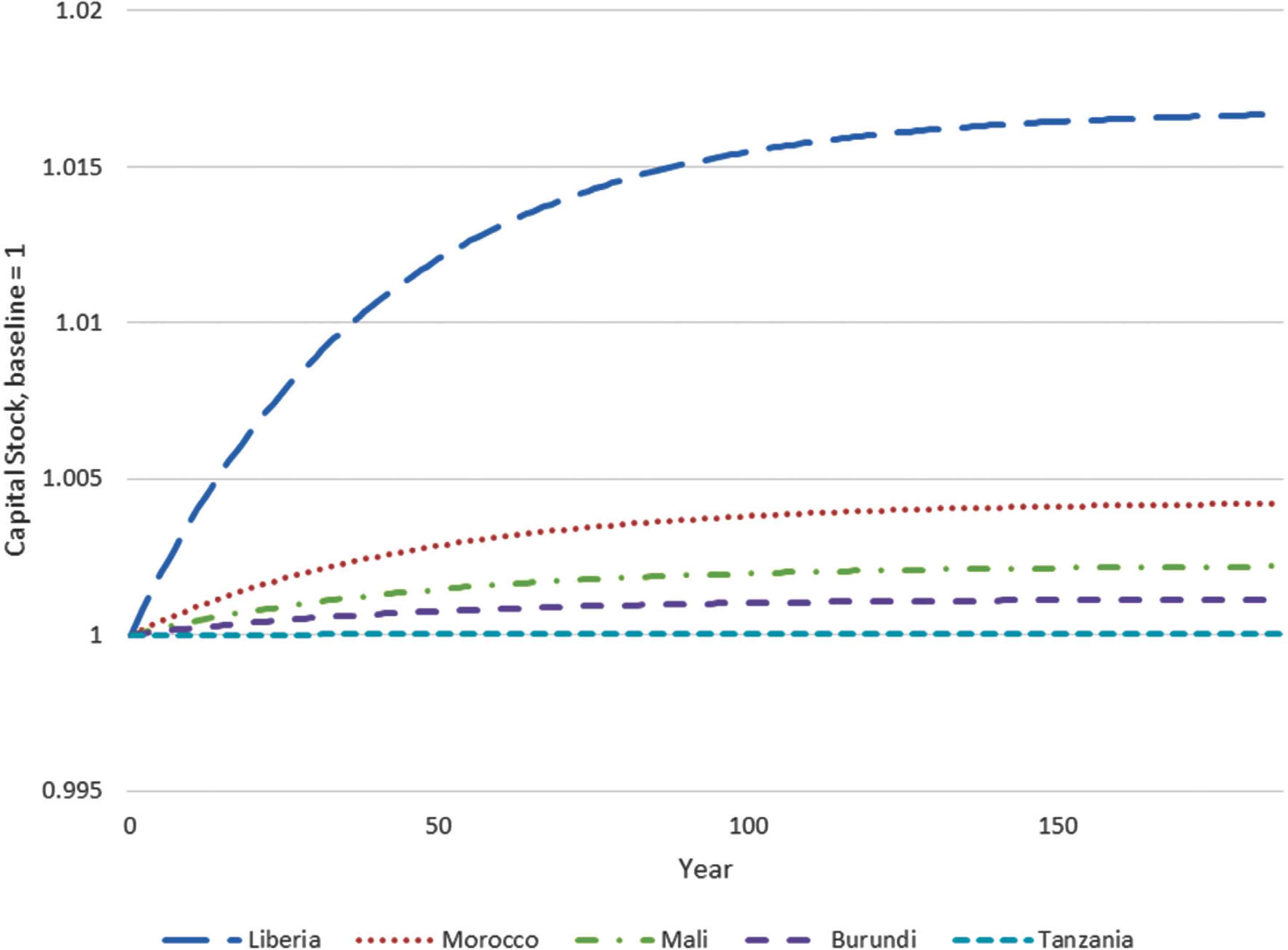
The evolution of capital stocks following AfCFTA.
Footnotes
The initial methodology was developed by Anderson et al. (2015a) in a static setting and augmented by dynamic general equilibrium (Anderson et al., 2015b) following the introduction of endogenous capital accumulation.
Yotov et al. (2016) provide a thorough description of the GEPPML process, starting from the theoretical reasoning up to the final stage, as well as practical guidelines for each of the steps. They also made available the code they used to implement the process on a large sample of countries. We adapted this code for our sample for the first three layers and developed the fourth layer. The original code is available at: https://vi.unctad.org/tpa/web/vol2/vol2home.html.
In addition, estimates found in other studies can be used; however, it is best to use the dataset in hand for both stages.
We drop one importer fixed effect per year to avoid perfect multicollinearity.
The pair fixed effects include internal trade γi,i, which is dropped due to perfect multicollinearity.
ER is the expenditure of Japan as the reference country.
Results with alternative parameter values are available upon request.
Due to poor data quality, we removed Syria from the sample, and replaced it with the United Arab Emirates.
CEMAC, COMESA, ECOWAS, EAC, WAEMU and SADC.
Available from: https://www.ewf.uni-bayreuth.de/en/research/RTA-data/index.html.
Another approach is to use period averages to account for business cycle fluctuations. Carrillo-Tudela and Li (2004) used 3-year averages for the same reason. Foster et al. (2011) used average trade flows 3 years prior and after the signing of a preferential free trade agreement. However, this approach can potentially bias the estimates (Bekkers, 2019).
Extracted from World Development Indicators (World Bank, 2020). Baier et al. (2019) present different methods to fill missing intra-national trade data, they found no significant discrepancy in results. Yotov et al. (2016) provide a discussion on the construction of intra-national trade data.
As a robustness test, we excluded EAC and WAEMU from the definition of major RTAs, for they are subsets of COMESA and ECOWAS. We ran the model with the results remaining virtually the same (not reported).
The actual share of intra-African trade is somewhat lower. Since we included the vast majority of African countries in the sample and excluded a lot smaller non-African countries, the estimated share is higher than the actual share.
However, to address the US structural current account deficits, the three countries members of the North American Free Trade Agreement (Canada, Mexico, and USA) reached a new agreement establishing the United States-Mexico-Canada (USMCA) as the successor of NAFTA in 2018.
The general equilibrium effects go from MRTs, to factory gate prices, to GDP. A fraction of change in GDP (governed by the Cobb–Douglas exponent) will go to capital accumulation, which will drive growth in future periods. Since the effect of MRTs is small given the size of African economies, the long-term effects are weak.
Maliszewska et al. (2020) provide a table with a summary of CGE studies on AfCFTA.
REFERENCES
Cite this article
TY  - JOUR
AU  - Hippolyte Fofack
AU  - Richman Dzene
AU  - Omar A. Mohsen Hussein
PY  - 2021
DA  - 2021/12/31
TI  - Estimating the Effect of AfCFTA on Intra-African Trade using Augmented GE-PPML
JO  - Journal of African Trade
SP  - 62
EP  - 76
VL  - 8
IS  - 2 (Special Issue)
SN  - 2214-8523
UR  - https://doi.org/10.2991/jat.k.211122.001
DO  - 10.2991/jat.k.211122.001
ID  - Fofack2021
ER  -