
Effect of exchange rate volatility on trade in Sub-Saharan Africa☆
- DOI
- 10.1016/j.joat.2017.12.002How to use a DOI?
- Keywords
- F1; F310; F320
- Abstract
The volatile nature of exchange rates with the advent of floating regimes has received much attention in economic research. The volatility is generally perceived as negatively affecting international trade. While theoretical predictions and empirical outcomes appear mixed, the balance seems to tilt in favour of this perception. Applying the pooled mean-group estimator of dynamic heterogeneous panels technique to data for eleven Sub-Saharan African economies over the period 1993 to 2014, this paper uncovers no significant effects of exchange rate volatility on imports. In the case of exports, however, the study finds a negative effect of volatility in the short-run, consistent with the above view, but a positive impact in the long-run.
- Copyright
- © 2017 Afreximbank. Production and hosting by Elsevier B.V. All rights reserved.
- Open Access
- This is an open access article under the CC BY-NC license (http://creativecommons.org/licences/by-nc/4.0/).
1. Introduction
The cessation of the Bretton Woods Monetary System of fixed parities, which has led to the adoption of floating regimes by many economies since 1973, has occasioned wide unpredictable fluctuations in bilateral exchange rates. These erratic movements have spawned renewed interest in exchange rates, owing to the perceived adverse effects on international trade (Dell’ Ariccia, 1999). The traditional school of thought holds that by intensifying the risk associated with cross-border exchanges, fluctuations in exchange rates may dampen the volume of international trade, as risk-averse traders substitute away from their high-risk trading obligations, towards less risky ones (McKenzie, 1999). The risk-portfolio stance, however, counters this traditional view, with the conjecture that higher risk implies higher returns. Thus, increasing risk due to fluctuating exchange rates could rather increase the volume of trade (De Grauwe, 1996).
In an ideal world where changes in exchange rates are predictable, volatility would not have significant adverse effects even if these changes were quite substantial. Traders may factor in the predicted changes by adjusting the agreed-on price, and as such, the observed movements in exchange rates would not impede trade (Hakkio, 1984). With floating regimes, however, movements in exchange rates have been highly unpredictable, thus often resulting in some undesirable and/or unpredictable influences on the balance of trade (Sosvilla-Rivero, 1999).
Balance of payments difficulties in developing countries date as far back as the 1970s, coming to a head in 1982 when Mexico declared the inability to service its debt. In the Sub-Saharan African (SSA) region, efforts to fix exchange rates despite external shocks with no support for fiscal and monetary policies, led to overvalued exchange rates with serious balance of payments consequences. Foreign exchange regimes of SSA economies were characterised by administrative controls on foreign exchange allocation and current account transactions, extensive foreign exchange rationing due to persistently weak external accounts, sizeable black market premiums and, notably, stagnating per capita real incomes (Maehle et al., 2013). In the 1980s and 1990s, many of these countries, in the face of severe macroeconomic imbalances, embarked on reforms to liberalise their economies. The reforms undertaken covered exchange rate and international trade liberalisation, in conjunction with structural reforms (Maehle et al., 2013).
Although exchange rate liberalisation was instrumental in the economic revival experienced by some SSA economies in the 1980s and 1990s, it has also led to an upsurge in exchange rate fluctuations. For instance, conditional variance plots of the generalized autoregressive conditional heteroskedasticity (GARCH) and exponential GARCH (EGARCH) models (see Fig. A1 in the Appendix) reveal significant levels of volatility over the periods following the exchange rate liberalisation of a group of 11 SSA floating economies. Consequently, it would be useful to examine the short- and long-run macroeconomic implications of a flexible regime with increasing exchange rate volatility, particularly in less developed economies. Has it effected adverse trade balance ramifications along the line? Evidence from the past two decades reveal a persistence in current account deficits, often exceeding the 5% ceiling in many floating developing economies (Osakwe and Verick, 2007). In a study of 38 SSA countries, spanning 1970 to 2005, Osakwe and Verick (2007) find that current account deficits in the region are driven principally by trade deficits. In addition, challenges often emerge in amassing inflows to counterbalance long running current account deficits (Osakwe and Verick, 2007). While a few economies are able to attract more stable sources of deficit financing, such as foreign direct investment (FDI) inflows, the majority depend on external debt, which may not be sustainable.
With persistent current account deficits and the challenges associated with their management, this paper examines the effects of exchange rate volatility on trade (exports and imports) in the SSA region. Although there are a large number of existing studies on the exchange rate volatility-balance of trade nexus on developing economies generally, a focus on Africa is important, given likely geographical differences. Existing studies on SSA countries have often been country-specific, and are unlikely to generate useful generalizable results. Consequently, this paper jointly covers 11 floating-exchange rate SSA economies1, namely, the Gambia, Ghana, Kenya, Madagascar, Mauritius, Mozambique, Nigeria, Sierra Leone, Tanzania, Uganda, and Zambia. The data spans 1993 to 2014. Using exchange rate volatility proxies generated by the GARCH and exponential GARCH models, and applying the pooled mean-group estimator of dynamic heterogeneous panels technique, the paper presents a multi-country analytical framework, and a regional outlook of the volatility impact on trade. The study uncovers no significant effects of exchange rate volatility on imports. In the case of exports, however, it finds a negative effect of volatility in the short-run, but a positive impact in the long-run.
The rest of the paper is organised as follows. The next section presents from the literature, theoretical underpinnings of the exchange rate volatility-trade nexus as well as a review of previous empirical studies. The econometric approach and a description of the data are contained in Section three, followed by analysis and interpretation of the empirical results in Section four. Section five concludes with implications for policy.
2. Exchange rate volatility and trade
The proposition that volatility in exchange rates has detrimental effects on trade flows earned formal grounding in Ethier (1973). Ethier’s model is centred on a risk-averse firm’s decision-making in relation to its imports and forward exchange cover in the face of uncertainty (volatility) in exchange rate movements. With the assumption of risk aversion, the trade response in the face of exchange rate volatility is deductively negative, although the significance of this inverse correlation diminishes with the speculative behavior of the firm (Ethier, 1973). Independently, Clark (1973) developed an analogous model of a firm with risk aversion producing inferences similar to Ethier’s model. The ‘risk aversion’ assumption, however, is not necessarily a precondition in the specification of a model that supports the adverse trade impact hypothesis (McKenzie, 1999). Demers (1991) modelled a competitive firm with risk neutrality in an environment where price uncertainty, resulting from exchange rate risk, leads to more uncertainty about the position or state of demand. With that much uncertainty, investment in physical capital is irreversible, resulting in declining levels of production and trade over time (Demers, 1991).
In contrast, other theoretical papers hypothesise a positive relationship between exchange rate volatility and trade. Franke (1991) modelled a risk-neutral firm in a monopolistically competitive market, maximising anticipated proceeds from its exports, where cash flow is defined as a positive function of the real exchange rate. In this analysis, the firm’s export strategy is key, determined by the transaction costs accrued. This cost is calculated via a comparison between the costs associated with entering or exiting a foreign market, and the profits or losses accumulated through exports. The assumption of a positive cash flow function in exchange rates implies that the rate of growth in the present value of cash flows exceeds costs incurred via entry and exit, and as such, the firm benefits with increasing exchange rate volatility. Predicted also is the idea that in the face of increasing exchange rate volatility, firms will hurriedly enter the said market to exploit the expected benefits and exit later (Franke, 1991). Bahmani-Oskooee and Hegerty (2007) review a number of theoretical papers postulating a positive effect of exchange rate volatility on the volume of trade. These papers include Viane and de Vries (1992), Sercu (1992), Sercu and Vanhulle (1992), Dellas and Zilberfarb (1993) and Broll and Eckwert (1999). Sercu (1992), for instance, shows that volatility could increase trade as it increases the probability that the price a trader receives might exceed trade costs. Sercu and Vanhulle (1992), on the other hand, theorise that rising volatility increases the value of exporting firms, thus encouraging exports. Viane and de Vries (1992) note the ambiguity of outcomes by observing that because importers and exporters are on opposite sides of a risky trading relationship, their respective roles are reversed, leading to a positive coefficient on the volatility variable for one partner. Broll and Eckwert (1999) also conclude that volatility increases the value of a trader’s option to export; since this risk increases the potential gains from trade, the volume of trade increases accordingly.
The ambiguity of the relationship between exchange rate volatility and trade flows is modelled by De Grauwe (1988), based on the supply decisions of a competitive firm. The firm is faced with the decision to sell either in a foreign or domestic market where prices are fixed. Consequently, the domestic currency price of exports appears the lone source of risk for the producer. In the absence of exchange rate risk diversification, the reaction of the producer to an upsurge in risk solely depends on the convexity or concavity of the expected marginal utility of export income function to exchange rates. In the event of lower risk aversion, less is produced for exports with increasing exchange rate volatility, on the premise that the marginal utility of export income is expected to fall. In the scenario of high risk aversion, however, exchange rate volatility increases the expected marginal utility of export income, thereby encouraging producers to increase production in attempts to evade severe decreases in their incomes.
In 1984, a decade following the collapse of the Bretton Woods system, the International Monetary Fund (IMF, 1984) pursued an inquiry into the economic influences of volatile exchange rates, specifically on international trade volumes. A survey and review of a decade’s worth of empirical literature characterised the intellectual exercise. Results revealed inconsistent outcomes, with many of the featured empirical studies finding little or no support for an inverse nexus. Plausible reasons adduced for the non-robustness of findings in these earlier studies include the inconclusiveness of theoretical inferences, as well as the use of relatively short sample periods with limited explanatory competences. Following the IMF’s 1984 study, renewed interest in the subject led to an explosion of empirical works seeking to understand the trade implications of volatile exchange rates. These assorted studies find evidence supporting both positive and negative hypotheses, as well as ambiguous outcomes. Studies confirming the negative hypothesis include Peree and Steinherr (1989), Bini-Smaghi (1991), Savvides (1992), Chowdhury (1993), Doganlar (2002), Clark et al. (2004), Mukherjee and Pozo (2011) and Khan et al. (2014). On the other hand, Klein (1990), Franke (1991), Sercu and Vanhulle (1992), McKenzie and Brooks (1997), McKenzie (1998), Doyle (2001), Bredin et al. (2003), and Kasman and Kasman (2005) find evidence in support of the positive hypothesis. The inconclusiveness of the relationship, however, is empirically affirmed by Gotur (1985), Bailey and Tavlas (1988), Bahmani-Oskooee and Sayeed (1993), Aristotelous (2001), Tenreyro (2007), and Osei-Assibey (2010).
Two decades following the IMF’s initial inquiry, Clark et al. (2004) re-examined the effect of exchange rate volatility on trade. They argue that some developments in the current global economy may have intensified fluctuations in exchange rates, while others may have lessened the influence of exchange rate volatility on trade. Liberalisation of capital flows, for example, is believed to have intensified exchange rate fluctuations, while the proliferation of the instruments of financial hedging may have lessened firms’ vulnerability to risks resulting from unpredictable currency movements. The impact of volatility on trade was found to be weakly negative. In a more recent study, Qureshi and Tsangarides (2011) also find a negative volatility impact on trade, significantly more in the long- run than in the short-run, where exchange rate volatility is defined as the standard deviation of the log first difference of the exchange rate.
On the SSA scene, only few studies have been carried out in relation to the exchange rate volatility-trade nexus, with a larger proportion being time series studies,2 relative to panel analysis. Osei-Assibey (2010) analyses the impacts of exchange rate volatility on trade flows in three Sub-Saharan African economies, namely, Ghana, Mozambique and Tanzania, with their respective trading partners, where volatility proxies are generated using the generalized autoregressive conditional heteroskedasticity (GARCH) model. Applying a gravity specification, he found the effect of volatility on trade earnings to be insignificant. Similarly, Akpokodje and Omojimite (2009) examine the effect of exchange rate volatility on the imports of ECOWAS (Economic Community of West African States) countries, where the GARCH model is used in generating the volatility series. A significant negative effect of exchange rate volatility on imports was realised in the pooled model comprising all ECOWAS economies. Outcomes on the sub-group of countries, however, were mixed. Whereas the non-CFA sub-group evidenced a negative correlation, positive volatility coefficients were obtained for the CFA sub-group.
The seemingly mixed results from empirical studies, while suggesting that the effect of exchange rate volatility on trade might be an empirical issue, may also reflect the vagueness of theoretical outcomes in the general equilibrium models; they allude to the fact that variability in exchange rates is contingent on the volatility of underlying shocks to policies, preferences, and technology, for example, in addition to the overall policy regime (Clark et al., 2004). In essence, fluctuations in exchange rate movements may be due simply to changes in the volatility of fundamental shocks and/or policy regimes, as suggested by the Driskill-McCafferty model (Grydaki and Fountas, 2009). Based on a relatively large sample of SSA countries and data that includes the more recent period, the present paper seeks to shed more light on the exchange rate volatility-trade nexus, particularly, in the context of SSA.
3. Empirical strategy
3.1. Model
To investigate the effect of exchange rate volatility on trade, export and import models are estimated in their long- and short-run specifications, incorporating pre-generated exchange rate volatility proxies, lags of each respective dependent variable to capture the influence of autoregressive components, and a pool of relevant explanatory variables. The export and import equations are specified as:
The adjustment coefficients α1, and β1 show how current exports and imports adjust to their immediate previous values respectively, and as such are expected to fall between 0 and 1 in absolute value. The exchange rate coefficient is expected to be negative for imports, but positive for exports, a priori. The real domestic income coefficient, however, is expected to bear positive sign for both imports and exports. With foreign reserves, nonetheless, the expectation is a positive coefficient for imports, but negative for exports. Inflation is expected to affect imports positively and exports negatively. Based on theoretical predictions and empirical outcomes, the signs of the coefficients of the GARCH and exponential GARCH (EGARCH) volatility proxies are expected to be ambiguous.
3.2. Estimation technique
The fixed and random effects estimators favour the conventional large N and small T panel framework. In their estimations, individual groups are pooled and only the intercepts are allowed to differ across panel units, thus assuming homogenous slope parameters. In recent years, attention has been drawn to dynamic panels with both large cross sectional and time series observations, owing to the use of data with higher frequency. The assumption of homogeneity of slope parameters often fails to hold with large N and large T dynamic panels (Pesaran et al., 1999). In this framework, however, the increase in time observations or large T inherently leads to the concern or realisation of non-stationarity, with series often integrated of order one. Consequently, Pesaran et al. (1997, 1999) make available two new approaches in the estimation of non-stationary dynamic panels with heterogeneous parameters across groups, namely, the mean-group (MG) and the pooled mean-group (PMG) estimators (Blackburne III and Frank, 2007). The MG estimator averages the coefficients of an estimated N time series regressions, whereas the PMG estimator depends on an amalgam of averaging coefficients arithmetically as well as pooling.
An autoregressive distributed lag (ARDL) dynamic panel model with i number of countries and t number of years, and with I(1) cointegrated variables, indicates an error term integrated of order zero for all panel units. Cointegrated variables are characterised by responsiveness to long-run equilibrium deviations, which fundamentally allude to an error correction model where the short-run dynamics of the variables in the model are affected by the deviation from equilibrium (Blackburne III and Frank, 2007). The MG and PMG models re-parameterise the ARDL dynamic panel model into an error correction model with an error-correcting speed of adjustment parameter ϕ. This model is estimated using the maximum likelihood estimator (ML), where ϕ is expected to be negative in suggestion of a return to long-run equilibrium following a deviation.
Accordingly, the paper applies the pooled mean-group (PMG) estimator of dynamic heterogeneous panels. Although alternative dynamic panel models such as the generalized method-of-moments (GMM), among others, have generated consistent coefficients in the circumstance of endogenous regressors, there is still the high plausibility of turning out misleading and inconsistent outcomes if slope coefficients fail to be truly or significantly identical across groups; which is often the case in most panel frameworks (Pesaran et al., 1999). However, the PMG model, which combines averaging and pooling, permits the error variances, intercept and short-run coefficients to differ across panel units, while constraining the long-run coefficients to be homogenous or equal across the spatial dimension (Pesaran et al., 1999)3. It is likely, that this estimation method will depict the true characteristics of the data and generate relatively more consistent and reliable average parameter estimates. The model is also able to provide both long- and short-run empirical estimates simultaneously. We test for unit root and cointegration using the Im-Pesaran-Shin test, and the Pedroni and Kao two-step residual based tests, respectively.
3.3. Data
Data frequency is annual, spanning 1993 to 2014, and is sourced from the World Bank’s World Development Indicators (see Appendix Table A1 for a description of the variables and their sources). In predicting conditional variances as proxy for volatility, the study uses the GARCH model, and one of its extensions, the exponential GARCH (EGARCH) model. Thus, we use two volatility proxies. The GARCH (1, 1) model accounts for volatility clustering, the property suggesting that volatility appears in clusters, and leptokurtosis, the property alluding to the fact that asset prices, such as exchange rates, are not mesokurtic. The GARCH (1, 1) model, however, fails to capture leverage effects - the stylized fact referring to the notion of a negative correlation between volatility and price movements - thus the need for the EGARCH model, which essentially captures the property. The EGARCH model, in capturing asymmetric effects, expresses conditional volatility logarithmically.
4. Results
Summary statistics of the variables employed are reported in Table A2 of the Appendix. Unit root tests4 reveal the stationarity of some variables at level and others at first difference, validating the need for a cointegration analysis in checking for constant co-variances over time. Cointegration tests5 indicate the presence of long-run equilibrium relationships among the variables of the system, and thus, the feasibility of a long- and short-run analysis. Overall, the results suggest a stable linear relationship between the dependent variables of the system and their respective explanatory variables in the long-run. Table A6 of the appendix presents the GARCH and EGARCH estimation results, indicating the presence of significant ARCH effects over the sample period; Fig. A1 captures country-specific graphical illustrations of the property of volatility clustering. The long- and short- run versions of Eqs. (1) and (2) are estimated twice, with the first estimation incorporating the GARCH based exchange rate volatility proxy, and the second estimation, using the EGARCH based exchange rate volatility proxy. Estimates for the long- and short-run export and import functions are presented in Tables 1 and 2, respectively.
| VARIABLE | Exports | Imports | ||
|---|---|---|---|---|
| 1 | 2 | 3 | 4 | |
| C | − 16.7432*** (4.2198) | − 12.4142*** (3.6687) | − 1.5694*** (0.2953) | 1.7354*** (0.3072) |
| lnEX−1 | 0.0680* (0.0341) | 0.0666* (0.0354) | ||
| lnIM−1 | 0.0499 (0.0307) | 0.0503 (0.0315) | ||
| lnEr | 0.0128 (0.0630) | 0.2120** (0.0925) | − 0.1232 (0.1319) | − 0.1416 (0.1278) |
| lnY | 1.1847*** (0.1169) | 1.1082*** (0.1291) | 0.1230 (0.3615) | 0.3703 (0.4261) |
| lnR | 0.2690*** (0.0524) | 0.2829*** (0.0575) | 0.6318*** (0.1226) | 0.8687*** (0.1357) |
| lnI | − 0.7946*** (0.0366) | − 0.7834*** (0.0456) | − 0.7014*** (0.0746) | − 0.7474*** (0.0744) |
| lnVol1 | 0.0568*** (0.0143) | 0.0339 (0.0275) | ||
| lnVol2 | 0.0134 (0.0135) | 0.0094 (0.0210) | ||
| Log likelihood | 144.0832 | 138.7004 | 1.8674 | 140.9415 |
Note: The dependent variables are the logs of real imports and real exports, *** and ** denote statistical significance at 1% and 5% respectively, figures in parentheses are standard errors, 1st regressions employ the GARCH based exchange rate volatility proxy, and 2nd regressions use the EGARCH based exchange rate volatility proxy.
Long-run export and import functions estimation.
Source: authors’ computation using STATA13.
| Variable | Exports | Imports | ||
|---|---|---|---|---|
| 5 | 6 | 7 | 8 | |
| C | − 16.7432*** (4.2198) | − 12.4142*** (3.6687) | − 1.5694*** (0.2953) | 1.7354*** (0.3072) |
| ln Δ EX−1 | − 0.0134 (0.0169) | − 0.0154 (0.0166) | ||
| ln Δ IM−1 | − 0.0253 (0.0213) | − 0.0254 (0.0213) | ||
| ln Δ Er | − 0.2135 (0.1411) | − 0.3432*** (0.1120) | − 0.5963*** (0.1090) | − 0.5414*** (0.1069) |
| ln Δ Y | 1.1641* (0.6268) | 1.1917** (0.5237) | 1.1661** (0.5736) | 1.0968** (0.4692) |
| ln Δ R | − 0.0338 (0.0414) | − 0.0149 (0.0398) | − 0.2336*** (0.0695) | − 0.2535*** (0.0685) |
| ln Δ I | − 0.4474*** (0.1622) | − 0.5841*** (0.1356) | − 0.6781*** (0.0480) | − 0.6617*** (0.0582) |
| ln Δ Vol1 | − 0.0675* (0.0389) | 0.0089 (0.0385) | ||
| ln Δ Vol2 | − 0.0473* (0.0253) | 0.0111 (0.0122) | ||
| Ec | − 0.6110*** (0.1534) | − 0.4633*** (0.1287) | − 0.3374*** (0.0526) | − 0.3292*** (0.0599) |
| Log likelihood | 144.0832 | 138.7004 | 1.8674 | 140.9415 |
Note: The dependent variables are the logs of the difference of real imports and real exports, *** and ** denote statistical significance at 1% and 5% respectively, figures in parentheses are standard errors, 1st regressions employ the GARCH based exchange rate volatility proxy, and 2nd regressions use the EGARCH based exchange rate volatility proxy.
Source: Authors’ computation using STATA13.
Short-run export and import functions estimation.
4.1. Exports
From Table 1, the GARCH exchange rate volatility proxy (model 1) is observed to affect exports positively in the long-run, significant at the 1% level. A 1% increase in exchange rate volatility thus increases real exports by 0.06%. This outcome conforms to Tenreyro (2007) and Hondroyiannis et al. (2008), who find a positive significant volatility effect on exports for a panel of 87 countries and G7 countries plus Switzerland, Norway, Ireland, Spain and Netherlands but differs with Chit et al. (2010), Arize et al. (2003), and Khan et al. (2014) who find evidence of a negative volatility impact for five emerging East Asian economies, thirteen least developed economies, and Pakistan’s trading partners. The significantly positive long-run estimate in our paper with respect to exports lends support to the positive propositions put forward by Franke (1991), Viane and de Vries (1992), Sercu (1992), Sercu and Vanhulle (1992), Dellas and Zilberfarb (1993) and Broll and Eckwert (1999).6 The control variables, namely, the nominal exchange rate, real domestic income and foreign reserves are observed to be positively correlated with exports while the effect of inflation is negative, in conformity with a priori expectations.
In the short-run (Table 2, models 5 and 6), however, both the GARCH and EGARCH volatility proxies provide evidence of an inverse correlation, albeit significant only at the 10% level. This may suggest that for these economies, real exports may be negatively affected by exchange rate volatility in the short-run, although this effect becomes positive in the long-run as reported above. A plausible explanation could be that at the instance of increasing volatility, risk-averse traders would instantaneously hold back on their high-risk exporting obligations in efforts to minimise probable trade losses. As time elapses, they are able to alter their inputs and overall production strategies towards maximising the benefits that accompany risky but profitable cross-border trading activities. A negative and statistically significant coefficient of the nominal exchange rate is observed in model 6, in adherence to the J-curve hypothesis. The expectation of a positive coefficient for real domestic income is affirmed. Foreign reserves failed to be significant at any of the conventional levels, even though it carried the expected negative sign. As expected, the rate of inflation evidenced negative coefficients, significant at the 1% level. Also, the expectation of a significant negative error correction term is achieved (models 5 and 6) at the 1% level. Specifically, about 46–61% of short-run adjustments occur annually towards long-run equilibrium.
4.2. Imports
In Table 1, results of models 3 and 4 (incorporating the GARCH and EGARCH volatility proxies, respectively) yield positive but insignificant coefficients in the long-run for import flows. Thus, for small import-dependent SSA economies, exchange rate volatility does not seem to significantly affect imports. Agolli (2003) also finds a positive relationship between exchange rate volatility and Albania’s imports from Germany and Greece, but with statistically significant coefficients. Khan et al. (2014), Akpokodje and Omojimite (2009), and Pugh et al. (1999), on the other hand, find a negative and significant impact of exchange rate volatility on long-run imports for Pakistan’s trading partners, a panel of ECOWAS countries, and 16 Organisation for Economic Co-operation and Development (OECD) countries. Foreign reserves are observed to be conformably positive and significant at the 1% level. The inflation rate posts negative and statistically significant coefficients, contradicting theoretical expectations. It is plausible that in the SSA region, inflationary pressures appear inversely related to import demand due to relatively higher currency depreciation, which could offset the gains or the desirability of a switch in preference towards foreign substitutes.
In the short-run, the volatility coefficients also bear positive signs but remain statistically insignificant (Table 2, models 7 and 8). The coefficient of the nominal exchange rate, however, produces statistically significant negative coefficients at the 1% level as expected a priori. Real domestic income yields positive coefficients, significant at the 5% level. Foreign reserves, however, bear an unexpected negative and significant coefficient, suggesting an inverse relationship between foreign reserves and real imports in the short-run. Similar to the long-run, the inflation rate maintained negative and statistically significant coefficients across both estimations, contradicting theoretical expectations. The error correction term posted the expected negative coefficient and is significant at the 1% level in both estimations, although adjustment is sluggishly achieved. Only about 33% of short-run deviations are corrected annually.
5. Conclusion and policy recommendation
This paper has examined the effects of exchange rate volatility on exports and imports based on a sample of 11 floating-exchange rate SSA economies, namely, the Gambia, Ghana, Kenya, Madagascar, Mauritius, Mozambique, Nigeria, Sierra Leone, Tanzania, Uganda, and Zambia, from 1993 to 2014. Using exchange rate volatility proxies generated by the GARCH and exponential GARCH models, the study uncovers no significant effect of exchange rate volatility on imports. In the case of exports, however, it finds a negative effect of volatility in the short-run, but a positive impact in the long-run. These results then indicate the differential impacts of exchange rate volatility between imports and exports and between the short-run and long-run, at least in the African context as represented by the sample of eleven counties. The positive impact on exports in the long-run is particularly welcome, especially as many African countries have adopted the floating exchange rate regime as part of economic reforms. These seemingly mixed results appear to complement the existing evidence in the literature that the effects of exchange rate volatility on trade might be an empirical issue; however, they may also reflect the vagueness of theoretical outcomes in the general equilibrium models.
As earlier noted, fluctuations in exchange rate movements may simply be due to changes in the volatility of fundamental shocks and/or policy regimes. Thus, policies that would help avoid the underlying causes of volatile exchange rate movements may be deemed more desirable than policies to moderate exchange rate fluctuations directly for trade expansion purposes. The unimpressive trade performance of most SSA economies might partly be attributed to macroeconomic shocks. Moderations in exchange rate volatility, therefore, may not necessarily yield significant positive effects on trade. The optimal control of fiscal and monetary shocks in support of growth may, however, also provide the stable economic environment for trade to thrive.
Appendix A
| VARIABLE | Description | Source |
|---|---|---|
| lnEX | Log of real exports of country i at time t | World Bank’s World Development Indicators |
| lnIM | Log of real imports of country i at time t | WDI |
| lnCF | Log of real FDI inflows into country i at time t | WDI |
| lnE | Log of nominal exchange rate of country i at time t | WDI |
| lnY | Log of real gross domestic product of country i at time t | WDI |
| lnR | Log of real foreign reserves of country i at time t | WDI |
| lnI | Log of inflation rate of country i at time t | WDI |
| lnVol1 | GARCH based exchange rate volatility proxy | Authors computation using STATA 13 |
| lnVol2 | EGARCH based exchange rate volatility proxy | Authors computation using STATA 13 |
Description and sources of variables.
| Variable | Mean | Standard deviation | Minimum | Maximum |
|---|---|---|---|---|
| Real exports (EX) (in millions of US$) | 79388.87 | 185568 | − 244463.7 | 1253803 |
| Real imports (IM) (in millions of US$) | 91060.11 | 227692.7 | − 536893 | 2753380 |
| Nominal exchange rate (E) (LCU per unit US$, period avg.) | 643.02 | 982.48 | 0.0649 | 4524.16 |
| Real domestic income (Y) (in millions of LCU) | 8.94e + 12 | 1.43e + 13 | 1.03e + 10 | 6.80e + 13 |
| Real foreign reserves (R) (in millions of US$) | 3.29e + 09 | 8.59e + 09 | 2.66e + 07 | 5.36e + 10 |
| Inflation rate (I) (annual %) | 13.92 | 16.47 | − 3.66 | 183.31 |
Source: authors’ computation using STATA13.
Descriptive statistics of variables, 1993–2014.
| Variable | Level | First difference | ||||
|---|---|---|---|---|---|---|
| t-Bar | t-Tilde-bar | Z-t-tilde-bar | t-Bar | t-Tilde-bar | Z-t-tilde-bar | |
| lnIM | − 1.834 | − 1.500 | − 0.445 | − 6.556*** | − 3.423*** | − 8.768*** |
| lnEX | − 1.791 | − 1.462 | − 0.278 | − 6.338*** | − 3.435*** | − 8.810*** |
| lnCF | − 2.096** | − 1.793** | − 1.677** | |||
| lnE | − 2.299** | − 1.876** | − 2.017** | |||
| lnY | 0.853 | 0.707 | 9.057 | − 1.110*** | − 4.115*** | − 11.62*** |
| lnR | − 1.247 | − 1.134 | 1.162 | − 10.43*** | − 3.771*** | − 10.15*** |
| lnI | − 2.844*** | − 2.344*** | − 4.032*** | |||
| lnVol | − 25.64*** | − 2.657*** | − 5.363*** | |||
Note: *** and ** denote stationarity at the 1% and 5% significance levels respectively.
Im-Pesaran-Shin (2003) panel unit root test results.
Source: authors’ computation using STATA 13.
| Model | Pedroni | Kao | |
|---|---|---|---|
| Panel ADF | Panel PP | Panel ADF | |
| Import function | − 5.8348*** | − 6.0594*** | − 6.6574*** |
| Export function | − 5.9979*** | − 9.2230*** | − 3.4010*** |
Note: *** denotes rejection of the null hypothesis at the 1% level of significance.
Pedroni and Kao residual cointegration tests results.
Source: Authors’ computation using EVIEWS 9.
| Ghana |
| Gambia |
| Kenya |
| Madagascar |
| Mauritius |
| Mozambique |
| Nigeria |
| Sierra Leone |
| Tanzania |
| Uganda |
| Zambia |
These are economies that have consistently allowed their currencies to float over the period the study covers. South Africa is excluded however, on grounds that the economy’s influence on empirical outcomes would be profound, owing to its relative largeness.
List of countries in the study.
| Variable | GARCH | Exponential GARCH | |||||||
|---|---|---|---|---|---|---|---|---|---|
| Constant | Arch | Garch | Constant (Arch) | Constant | Earch | Earch_a | Egarch | Constant (Arch) | |
| Ghana | 90.3544*** (0.2663782) | 1.0393*** (0.2969294) | 0.0593 (0.093082) | 1.5344** (0.7959) | 90.2531*** (0.1989) | 0.1278 (0.2328) | 1.9820*** (0.3596) | 0.8603*** (0.0754) | 0.3520 (0.3039) |
| Gambia | 85.6548*** (0.2044) | 0.9895*** (0.1825) | 0.0755 (0.0543) | 1.6385*** (0.5935) | 86.5544*** (0.1406) | 0.1111 (0.1730) | 1.8721*** (0.2543) | 0.8823*** (0.0539) | 0.3401* (0.1975) |
| Kenya | 92.9148*** (0.8631) | 1.0985* (0.6456) | −0.0870 (0.2688) | 9.4591 (7.3527) | 90.6766*** (0.4243) | 0.0576 (0.5028) | 2.4093** (0.9659) | .8935*** (0.2641) | 0.2242 (1.1892) |
| Madagascar | 110.2232*** (0.2344) | 1.0546*** (0.2034) | 0.0100 (0.0986) | 5.8188 (2.4565) ** | 105.4111*** (0.3609) | 0.9242 (0.2220) | 1.0400** (0.2327) | 0.2251*** (0.1498) | 1.5662*** (0.8242) |
| Mauritius | 103.8231*** (0.1823) | 1.0395*** (0.3021) | −0.0606 (0.0734) | 1.8720*** (0.7168) | 104.2364*** (0.1664) | 0.0886 (0.3090) | 2.0364*** (0.4450) | 0.6417*** (0.1184) | 0.8576** (0.3381) |
| Mozambique | 98.5696*** (0.3894) | 0.9557*** (0.2922) | −0.0956 (0.0806) | 19.4886*** (6.9784) | 106.2351*** (0.3741) | −0.1821 (0.1867) | 1.5996*** (0.2938) | 0.6354*** (0.0982) | 1.4429*** (0.4010) |
| Nigeria | 96.8395*** (0.3501) | 0.8605*** (0.3281) | 0.1655** (0.0793) | 1.7574** (0.7265) | 96.8624*** (0.3540) | 0.7888 (0.4905) | 0.1787** (0.6199) | 0.6199*** (0.0867) | 1.7491 (0.7184)** |
| Sierra Leone | 103.1407*** (0.5739) | 1.0361** (0.5745) | 0.0689 (0.6162) | 0.1746* (0.4504) | 100.1841*** (0.4292) | 0.4858 (0.3506) | 0.5861*** (0.5631) | 0.0020 (0.1361) | 1.9724*** (0.4603) |
| Tanzania | 111.7895*** (2.3555) | 1.240* (0.7085) | −0.0656 (0.4626) | 0.0017 (0.0149) | 113.5853*** (2.3356) | 0.5338 (0.8407) | 2.3052** (1.0822) | 0.6525*** (0.1833) | 2.0066 (1.2670) |
| Uganda | 101.744*** (0.2222) | .8931** (0.3729) | 0.1655 (0.1122) | 1.5773* (0.8521) | 101.8515*** (0.1689) | 0.0346 (0.1946) | 1.5555*** (0.3402) | 0.8826*** (0.0649) | 0.2715 (0.2218) |
| Zambia | 102.2528*** (0.3091) | 1.1040*** (0.1892) | −0.0384 (0.0567) | 6.1666*** (1.6473) | 102.2067*** (0.1313) | −0.2257 (0.1604) | 1.5351*** (0.2037) | 0.8125*** (0.0775) | 0.7261*** (0.2600) |
Note: Estimations were based on monthly real effective exchange rates data spanning 1995 m1 to 2017m5, and sourced from Bruegela datasets. Figures in parentheses reflect standard errors, and ***, **, and * denote statistical significance at 1%, 5% and 10% respectively.
Bruegel is an independent international economic policy research think tank, based in Brussels, Belgium. http://bruegel.org/publications/datasets.
GARCH and EGARCH country-specific volatility results.a
Source: Authors’ computation using STATA13.
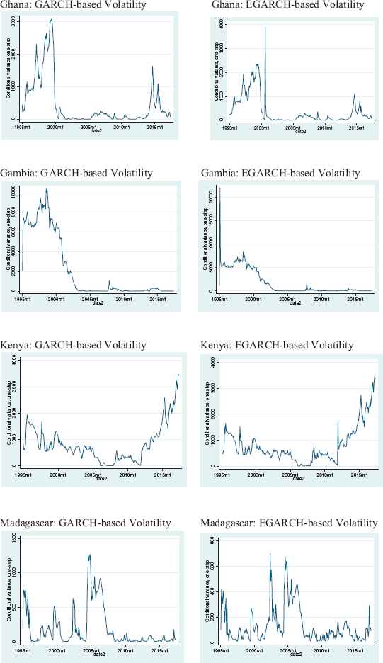
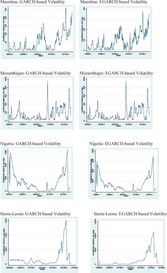
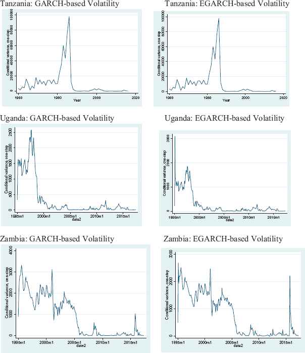
Country-specific conditional variance (volatility) plots.
Footnotes
We would like to thank Prof. Augustin K. Fosu (Editor-in-Chief of this journal) and the anonymous reviewer(s) for their helpful comments on earlier versions of the paper. Errors and omissions are the sole responsibility of the authors.
These are economies that have consistently allowed their currencies to float over the period covered by the study. We however exclude South Africa from our country sample on the evidence of it being an outlier, which would lead to biased and inefficient estimates.
See for instance, Aliyu (2010), Obi et al. (2013), Nyahokwe and Ncwadi (2013), and Modisaatsone and Motlaleng (2013).
See Pesaran et al. (1999) for a detailed theoretical account on the pooled mean-group model.
References
Cite this article
TY  - JOUR
AU  - Bernardin Senadza
AU  - Desmond Delali Diaba
PY  - 2018
DA  - 2018/02/18
TI  - Effect of exchange rate volatility on trade in Sub-Saharan Africa☆
JO  - Journal of African Trade
SP  - 20
EP  - 36
VL  - 4
IS  - 1-2
SN  - 2214-8523
UR  - https://doi.org/10.1016/j.joat.2017.12.002
DO  - 10.1016/j.joat.2017.12.002
ID  - Senadza2018
ER  -