
Deep Learning for Detection of Routing Attacks in the Internet of Things
- DOI
- 10.2991/ijcis.2018.25905181How to use a DOI?
- Keywords
- deep learning; continuous monitoring; cyber-physical systems; cyber security
- Abstract
Cyber threats are a showstopper for Internet of Things (IoT) has recently been used at an industrial scale. Network layer attacks on IoT can cause significant disruptions and loss of information. Among such attacks, routing attacks are especially hard to defend against because of the ad-hoc nature of IoT systems and resource constraints of IoT devices. Hence, an efficient approach for detecting and predicting IoT attacks is needed. Systems confidentiality, integrity and availability depends on continuous security and robustness against routing attacks. We propose a deep-learning based machine learning method for detection of routing attacks for IoT. In our study, the Cooja IoT simulator has been utilized for generation of high-fidelity attack data, within IoT networks ranging from 10 to 1000 nodes. We propose a highly scalable, deep-learning based attack detection methodology for detection of IoT routing attacks which are decreased rank, hello-flood and version number modification attacks, with high accuracy and precision. Application of deep learning for cyber-security in IoT requires the availability of substantial IoT attack data and we believe that the IoT attack dataset produced in this work can be utilized for further research.
- Copyright
- © 2018, the Authors. Published by Atlantis Press.
- Open Access
- This is an open access article under the CC BY-NC license (http://creativecommons.org/licences/by-nc/4.0/).
1. Introduction
The term of Internet of Things (IoT) is a system of interconnected devices, machines and related software services. IoT plays an important role in the modern society since it enables energy efficient automation for enhancing quality of life. However IoT systems are an obvious target for cyber-attacks because of their ad-hoc and resource-constrained nature. Therefore, continuous monitoring and analysis are needed for securing IoT systems. For the security monitoring and analysis of IoT, forecasting malicious attacks is crucial to adapt with unexpected conditions, take precautions, protect sensitive data, provide continuity and minimize possible losses. Because of the vast amount of network and sensing data produced by IoT devices and systems, Big Data and machine learning methods are highly effective in continuous monitoring and analysis for security of IoT systems.
In this study we propose a highly-scalable deep-learning based attack detection method for routing attacks in realistic IoT scenarios. We obtained a high degree of training accuracy (up to 99.5%) and F1-scores (up to 99%). In this study, we have focused on specific I oT r outing a ttacks, n amely, decreased rank, version number modification and hello-flood. We have generated an IoT Routing Attack Dataset, named IRAD, with size close to 64x106 which allows for successful deep-learning based attack detection in IoT.
Traditional machine learning methods, such as Bayesian Belief Networks (BBN)1, Support Vector Machines (SVM)2,3,4,5 and others6,7,8,9 have been applied for cyber security. However, IoT systems generate a large size of data, and the classical machine learning methods tend to decrease in performance and scalability when the data size gets larger. In contrast, deep learning based machine learning performs better when trained with large data sizes and is adaptable to different attack scenarios, since deep learning can derive features from initially provided features (sometimes also called meta-features).
IPv6 is a commonly used protocol in IoT and IPv6 based wireless sensor networks (WSNs)10 are particularly susceptible to routing attacks. IPv6 over Low-powered Wireless Personal Area Networks (6LoW-PAN) is an IPv6 based WSN protocol11. 6LoWPAN has some advantages such as low power consumption, tiny, small foot print, inexpensive structure and easy maintenance12. Besides, WSNs include many sensors which have limited resources such as low memory, small bandwidth and low energy. A depiction of routing attacks against IoT systems can be found in Figure 1.
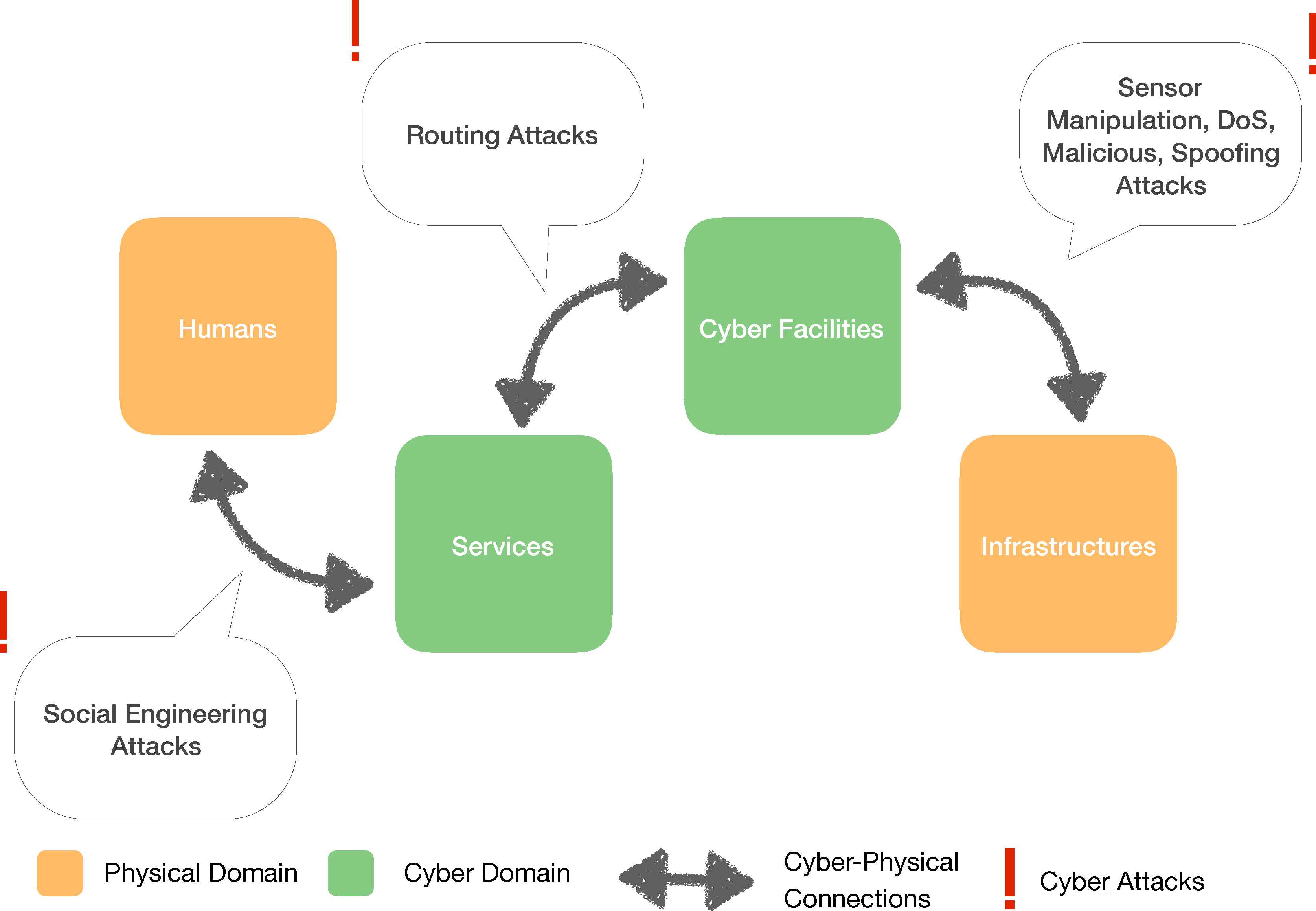
An overview of IoT attacks
In this study the viability of the proposed methodology has been validated by using up to 1000 nodes. Existing studies13,14,15 have demostrated their methodology using a small number of nodes (10-50), which is not a realistic approach for a real IoT environment.
Our proposed methodology is depicted in Figure 2. We have generated data by real-life equivalent simulations using the open source Contiki/Cooja simulator 16, because of lack of availability of public IoT attack data sets. The Cooja simulation generates raw packet capture (PCAP) files, which are first converted into Comma Separated Values (CSV) files for text-based processing. The CSV files are then fed into the feature pre-processing module of our system. The features are calculated based on the traffic flow information in the CSV files. First, a feature extraction process takes place. Thereafter, feature normalization is applied to all datasets to reduce the negative effects of marginal values. In the pre-feature selection step, as a result of feature importance analysis, some of the features are dropped.
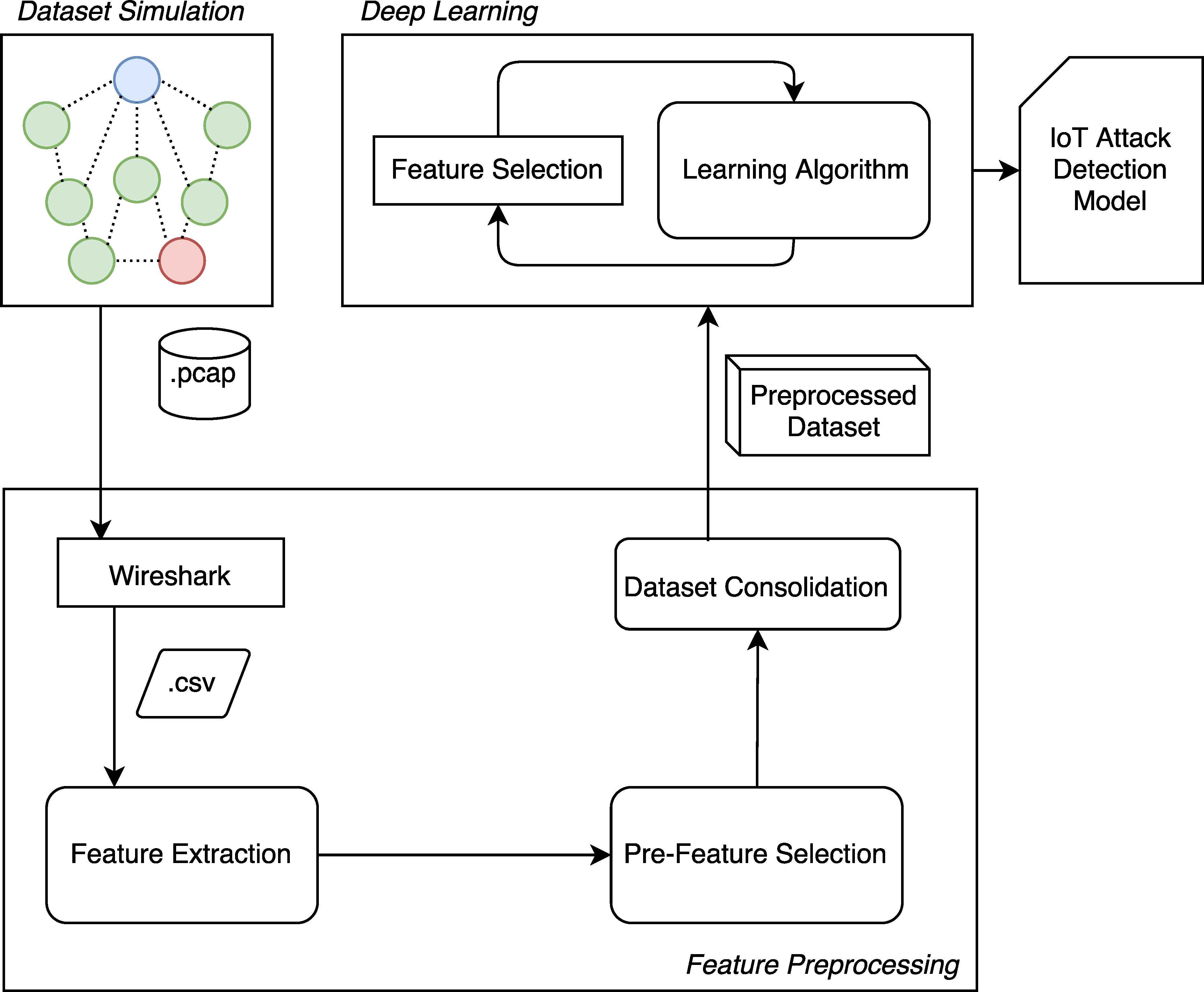
Methodology Flow Diagram
After feature pre-processing, the datasets corresponding to each scenario are labelled and mixed. As a result, preprocessed dataset is produced, consisting of a mixture of attack and benign data. These datasets are fed into deep learning algorithm. Deep layers are trained with regularization and dropout mechanisms, their weights are adjusted and the IoT Attack Detection Models are created.
IoT devices are resource constrained and have power consumption limitations. As a result of these constraints the security mechanisms devised for IoT should be efficient and lightweight, putting ver small computation and communication burden on the end-devices as possible. Our proposal puts minimum burden on the IoT network since it requires only the network packet traces for detection and prediction of attacks which can be collected externally by network recording equipment or specially designated nodes. According to the best our knowledge, this is the first study which uses deep learning based methodology for routing attack detection in IoT network.
Deep learning requires significant amount of data for efficient training. In this research area, lack of datasets is one of the biggest challenges. So we simulated the routing attacks within different scenarios and processed raw datasets to make them ready for detection process. Finally we concatenate the same attack datasets to make a comprehensive dataset. Thus, three IoT attack datasets were obtained. The details of mentioned scenarios and datasets are listed in Table 1.
| Malicious | Benign | ||||||
|---|---|---|---|---|---|---|---|
| Datasets | Scenarios | Nodes | Mal./Ben. Nodes | Total Packets | Scenario | Nodes | Total Packets |
| Decreased Rank | DR10 | 10 | 2/8 | 130.240 | Benign10 | 10 | 121,047 |
| DR20 | 20 | 4/16 | 398,143 | Benign20 | 20 | 120,897 | |
| DR100 | 100 | 10/90 | 456,816 | Benign100 | 100 | 150,078 | |
| DR1000 | 1000 | 100/900 | 801,396 | Benign1000 | 1000 | 739,845 | |
| Hello Flood | HF10 | 10 | 2/8 | 100,538 | Benign10 | 10 | 121,047 |
| HF20 | 20 | 4/16 | 104,302 | Benign20 | 20 | 120,897 | |
| HF100 | 100 | 10/90 | 300,986 | Benign100 | 100 | 150,078 | |
| HF1000 | 1000 | 100/900 | 1,739,226 | Benign1000 | 1000 | 739,845 | |
| Version Number | VN10 | 10 | 2/8 | 112,044 | Benign10 | 10 | 121,047 |
| VN20 | 20 | 4/16 | 203,153 | Benign20 | 20 | 120,897 | |
| VN100 | 100 | 10/90 | 223,275 | Benign100 | 100 | 150,078 | |
| VN1000 | 1000 | 100/900 | 1,585,075 | Benign1000 | 1000 | 739,845 | |
Details of Datasets
The rest of the paper is organized as follows: Section 2 presents related work about IoT attack detection by using different approaches. Section 3 gives detailed information about this research: Routing Attacks and Features for Deep Learning, Simulation of IoT Attacks, Dataset Generation and Feature Extraction, Feature Normalization, Feature Selection and Deep Learning. In Section 4, results and analysis of the research are given. Discussion and Conclusions are given in Section 5.
2. Related Work
Designing and ensuring sustainability of secure IoT systems the best way is to protect against malicious attacks before they happen. At this point, detecting and if possible, predicting malicious attacks come into prominence to protect the IoT systems against attacks. There are two alternative approaches for attack detection; rule-based (or signature-based) approach and predictive (or behavioural) approach. Signature based solutions fail against routing attacks that have changed their nature slightly. The anomaly detection methods are better than signature based solutions for the detection accuracy of previously unseen attacks.
There are several studies on routing protocol attack detection for IoT using the rule-based approach. In research of Raza et al. 17, node IDs and ranks are checked to matching assigned values for detecting anomalies. If a malicious node is detected, an alarm is raised. However rule-based detection isn’t efficient for complex systems and unidentified attacks because many rules are required which brings management difficulty of rules. Additionally, since rules are derived from pre-determined system configurations and known attacks, new rules need to be added to deal with new type of attacks.
Avram et al. 18 aim to detect routing attacks by using Self Organizing Maps (SOM) algorithm. For the AODV routing protocol, they created scenarios, benign and mixed, to calculate the proposed system accuracy. Their algorithm detects some routing attacks with high accuracy, nevertheless the study suffers from a high false positive rate (9.5%).
Banković et al. 15, researchers aim to detect unknown attack in WSN. In the centralized routing tree, there are some PDA-like sensors, that have more power resource and computational capacity to solve node’s constraints issue. They aim to detect the Sybil attack, a kind of routing attack that malicious nodes try to impersonate from other nodes. Their proposed algorithm has been tested on a 40-node WSN, gets high detection rate until the percentage of malicious nodes exceed 52%.
Pongle et al. 13 studied on detecting wormhole attacks in IoT. Wormhole attack is topology based routing attack that aim to affect network topology and packet traffic flows. Their proposed IDS-based detection system identify the wormhole attacks by using node’s and neighbour’s location and also identify attacker node by using received signal strength. They focus on RPL as the routing protocol and simulate the IoT network by using Cooja. Their network topology has up to 24 nodes. The number of nodes is not realistic for real IoT environment. Likewise, Nait-Abdesselam et al. 14 proposed a rule-based detection system. They use OLSR19, as routing protocol, and NS-2 simulator20 for creating network. In the study of Nait-Abdesselam et al. 14, the number of nodes is more than other studies13, as 10 to 50 nodes.
Dhamodharan et al. 21 aim to detect the Sybil attack. In the Sybil attack, attacker temporarily uses different (normal) node’s identity while communicating with neighbour nodes. They create network, that based on AODV protocol, by using NS-2 simulator 20. Message authentication is applied to detect Sybil nodes, as a rule-based solution.
The usage and efficiency of various Machine Learning(ML) and data mining methods for intrusion detection is discussed by Buczak et al. 6. ML result metrics (False Positive, False Negative etc.), core ML methods (SVM, Bayesian, Decision Tree, Clustering etc.), complexity of the ML methods used on public datasets and features of the datasets are discussed.
As an example of SVM, in the research of Chowdhury et al. 9, ten subsets of data set features are created randomly by feature selection, where one of the subsets contains three features. Then, these feature subsets are input to the SVM algorithm respectively. The authors claim to improve detection accuracy from 88.03% to 98.76% as a result by using one of the feature subsets instead of using all features.
Janakiram et al. 1 also applied BBN algorithm to detect outliers in WSN but these studies has no contribution about routing attacks.
There are some applications of SVM to IoT. SVM is an supervised ML model for solving classification and regression problems. The researchers proposed outlier detection systems in WSN. However these studies3,4,5,2 don’t address routing attacks.
In the study of Kaplantzis et al. 3, researchers aim to build a simple classification based IDS to detect selective-forwarding attacks. IDS generates an alarm depending upon bandwidth and hop count thresholds. The classification process is designed by using SVM classifiers. Determined features, bandwidth and hop count, can produce accurate results for the blackhole attack, but for other routing attacks, they are not as efficient.
Diro et al. 22, proposed deep learning based distributed attack detection for IoT. They also compare the traditional machine learning with deep learning about performance of distributed attack detection. Distributed attack detection is done by fog computing23 in this study. They also used NSLKDD24 dataset for detecting attacks. Although this study is a promising approach for distributed deep learning, but does not address IoT attacks specifically.
3. Deep Learning Based Detection of Routing Attacks
Diro et al. 22 stated in their research that deep learning which involves multiple hidden neural network layers has better performance than shallow learning, which involves only one hidden neural network layer. Deep learning performs better with larger data sizes and since it is more adaptable to varying parameters in the data. IoT systems produce large data sizes and the attacks against IoT systems show varying characteristics which are not easily detectable by linear models. In contrast, there are also some drawbacks such as inclined to overfitting25 or distinctive solutions, according to “no free lunch theorem”(NFLT)26, that means a solution for specific problem is useless for another problem. Nevertheless, deep learning is a promising machine learning method for detection and prevention of attacks against IoT systems.
In our methodology, first wireless traffic packet capture files for various benign and attack scenarios are generated using the Cooja simulator. Features are extracted from the packet capture files based on the characteristics of the IoT routing attacks. The importance of the features are evaluated due to the datasets’ index for selecting features to make the learning process more accurate. The features with too high and low importances are dropped in order to help prevention of over-fitting and under-fitting during training. The datasets are normalized by a feature normalization process to make the training process faster. The output of the feature pre-processing step are pre-processed datasets which are taken into deep learning algorithm. The learning algorithm is implemented by the help of Python libraries such as KERAS (available at: https://keras.io), Scikit27 and Numpy28. The learning process outputs the IoT attack detection model. We tested the model against multiple test scenarios for a more accurate measurement of precision and recall.
3.1. Simulation of IoT Attacks
In order to obtain a highly generalizable neural network model, network communication data corresponding to a variety of IoT scenarios, with and without malicious nodes, need to be obtained. For this purpose, we utilized the Cooja IoT simulator to simulate different IoT network communication scenarios. Cooja, coupled with the Contiki operating system, is a cross-layer (application, operating system and machine code layer) simulation tool16. Sensors in the simulated network run with the Contiki operating system and implement the RPL protocol. Contiki makes possible to load and unload individual programs and services to simulated sensors29. We have conducted a simulation of each attack as mentioned above, by running real sensor code in Cooja simulator, in a virtual machine with 48 GB RAM and 8 VCPUs on a private cloud. We opted for using the cloud infrastructure since simulations from 100 up to 1000 nodes require high memory and computing power. The Contiki environment includes 64-bit Java Runtime Environment on top at 64-bit Ubuntu operating system and Contiki 3.0. A sample of IoT simulation is shown in Figure 3.
A sample of the Simulation
We built different network topologies for simulating IoT routing attacks. We simulated these scenarios by the Cooja network simulation, at the same time, avoiding to produce a synthetic dataset, since Cooja enables to run actual RPL code on the simulated nodes. Cooja allows taking transmitted radio messages in the simulated network as a PCAP file. Subsequently, we transform the PCAP file to CSV with the help of our Python data preprocessing library. After that, a feature extraction process is applied to the generated CSV files.
After the scenarios were simulated, the datasets were produced as PCAP files. We dissected the PCAP file into CSV by using Wireshark and input to pre-processing. A sample of raw dataset is shown in Table 2.
| No. | Time | Source | Destination | Length | Info |
|---|---|---|---|---|---|
| 4755 | 14.611416 | fe80::c30c:0:0:12 | fe80::c30c:0:0:11 | 102 | RPL Control (DODAG Information Object) |
| 4756 | 14.611886 | fe80::c30c:0:0:8 | ff02::1a | 97 | RPL Control (DODAG Information Object) |
| 4757 | 14.612891 | fe80::c30c:0:0:4 | fe80::c30c:0:0:18 | 76 | RPL Control (Destination Advertisement Object) |
A Sample of Raw Dataset
3.2. Routing Attacks and Features for Deep Learning
Routing Protocol for Low-Power and Lossy Networks (RPL)30 is a tree-oriented IPv6 routing protocol for 6LoWPAN. It creates Destination Oriented Directed Acyclic Graphs (DODAGs), called as DODAG tree. Each network has one or more DODAG root node as central node and each network has a unique identifier DODAG ID to be identified. Additionally, each node has a rank number and a routing table due to the other nodes’ rank numbers. The rank number is used to determine the distance between the node and root31.
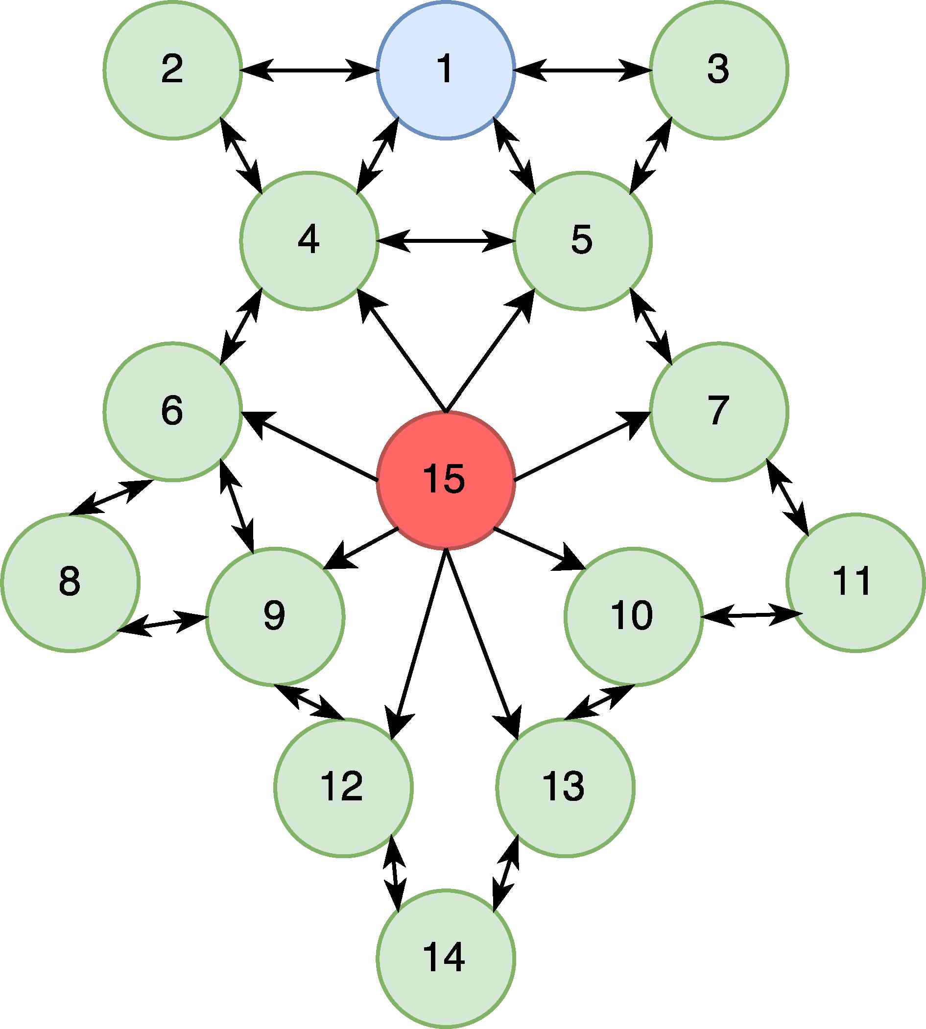
In the RPL protocol, there are three type of control packets; DODAG Information Object (DIO), Destination Advertisement Object (DAO) and DODAG Information Solicitation (DIS). DIO packets are first sent by base (or root) node as broadcast packets to establish the DODAG tree. The rest of the nodes receive the DIO packets and they create their routing table by selecting their parent node. They send DAO packets to the parent node, asking permission to connect to the parent node. The parent node accepts this offer by sending back a DIO ACK packet. A new node sends DIS packets to join the DODAG tree. If a new node joins the tree, all nodes send DIO packet again to reform DODAG (or network topology). An example of RPL network is depicted in Figure 4.
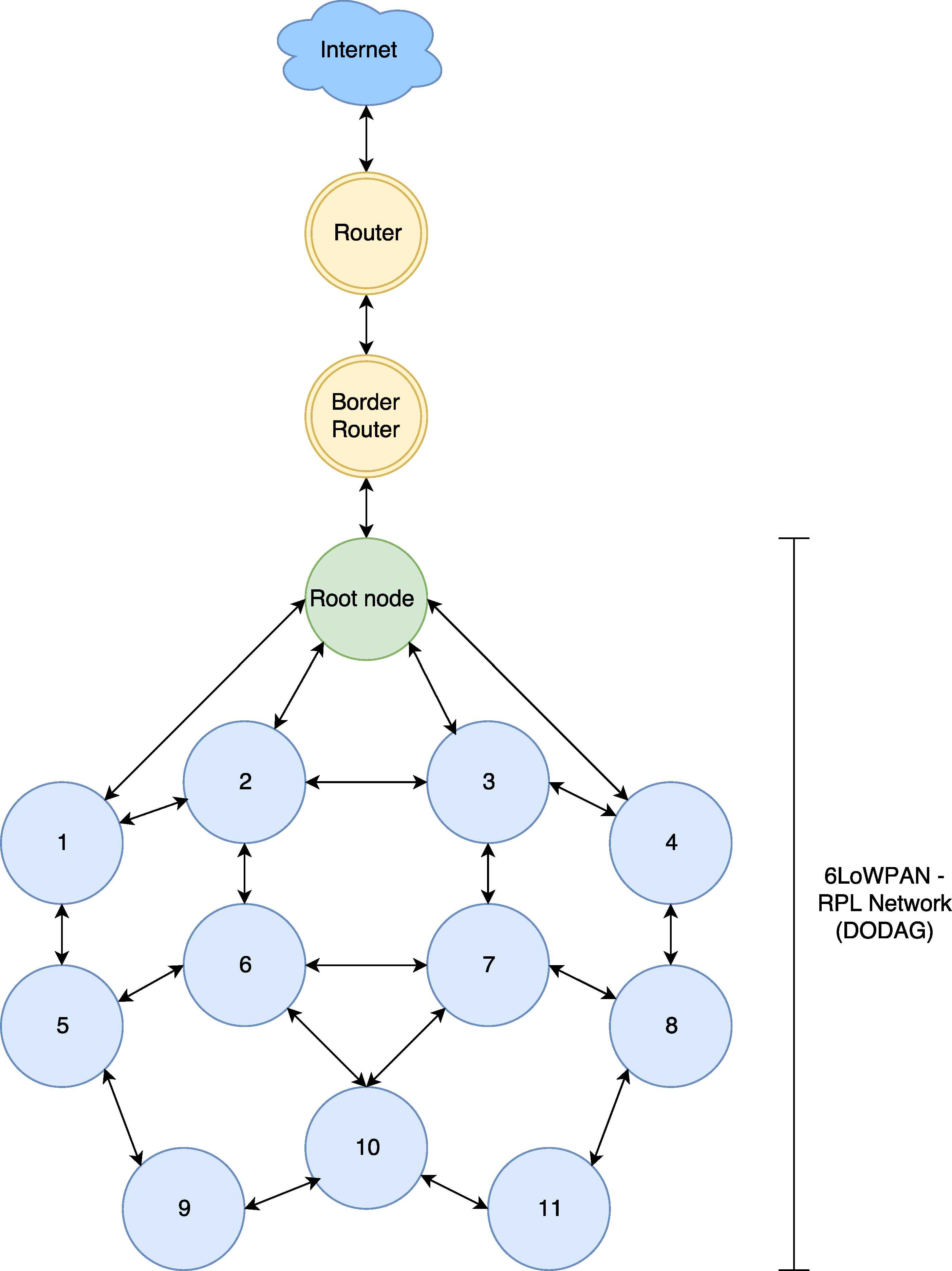
Sample 6LoWPAN Concept
Routing attacks take place at the network layer. Among the most significant routing attacks are decreased rank (DR), hello-flood (HF) and version number modification (VN) attacks.
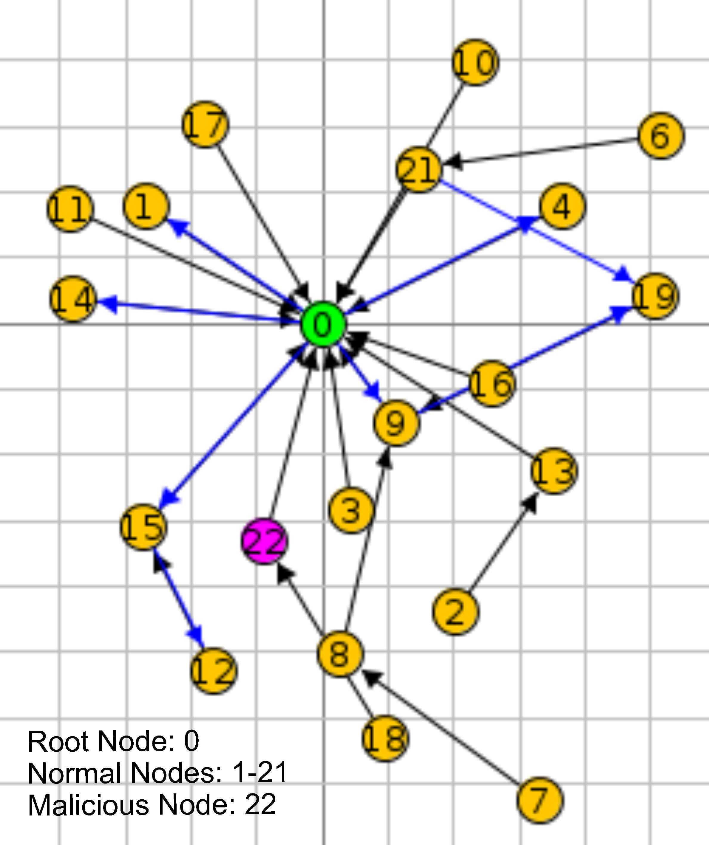
The DR attack is a kind of traffic misappropriation attack. In this kind of attack, malicious nodes advertise a rank lower than the other nodes to their neighbour nodes, by sending DIO packets. As a result, the neighbour nodes change their routing path to include attacker node by sending DAO packets. DR attack can be applied as a preparation for black hole, eavesdropping and sink hole attacks. DR attack is depicted in Figure 5. In this figure, Node 1 is the DODAG root node and the others are normal nodes. The nodes, 3 to 8, are not effected by the attack. Node 9 is the malicious node that conducts the DR attack. Nodes 10 and 11 are partially affected from the attack. Some of the packets originating from these nodes could be received by the malicious node because the malicious node is in their routing table, i.e., the other nodes send their packets through the malicious node. The nodes, 12 to 18, are the victim nodes whose communication is transmitted over the malicious node.
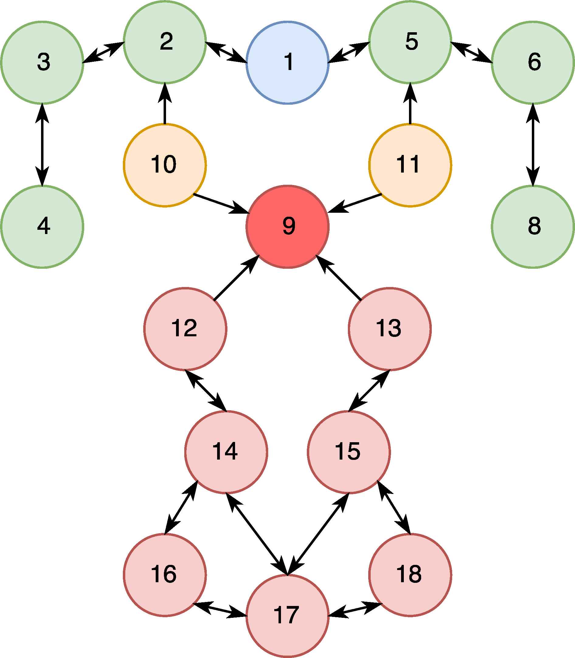
Decreased Rank Attack
It is evident that number of received packets of the malicious node increases when this attack happens. We aim to use this anomaly as a feature. Accordingly, Reception Rate (RR) (1), Reception Average Time (RAT) (2), Received Packets Counts (RCP), Total Reception Time(TRT) statitistics are calculated, per transmission window (1000 ms). Additionally, DIO and DAO packet counts are calculated because of the the attack is carried over DIO and DAO packets.
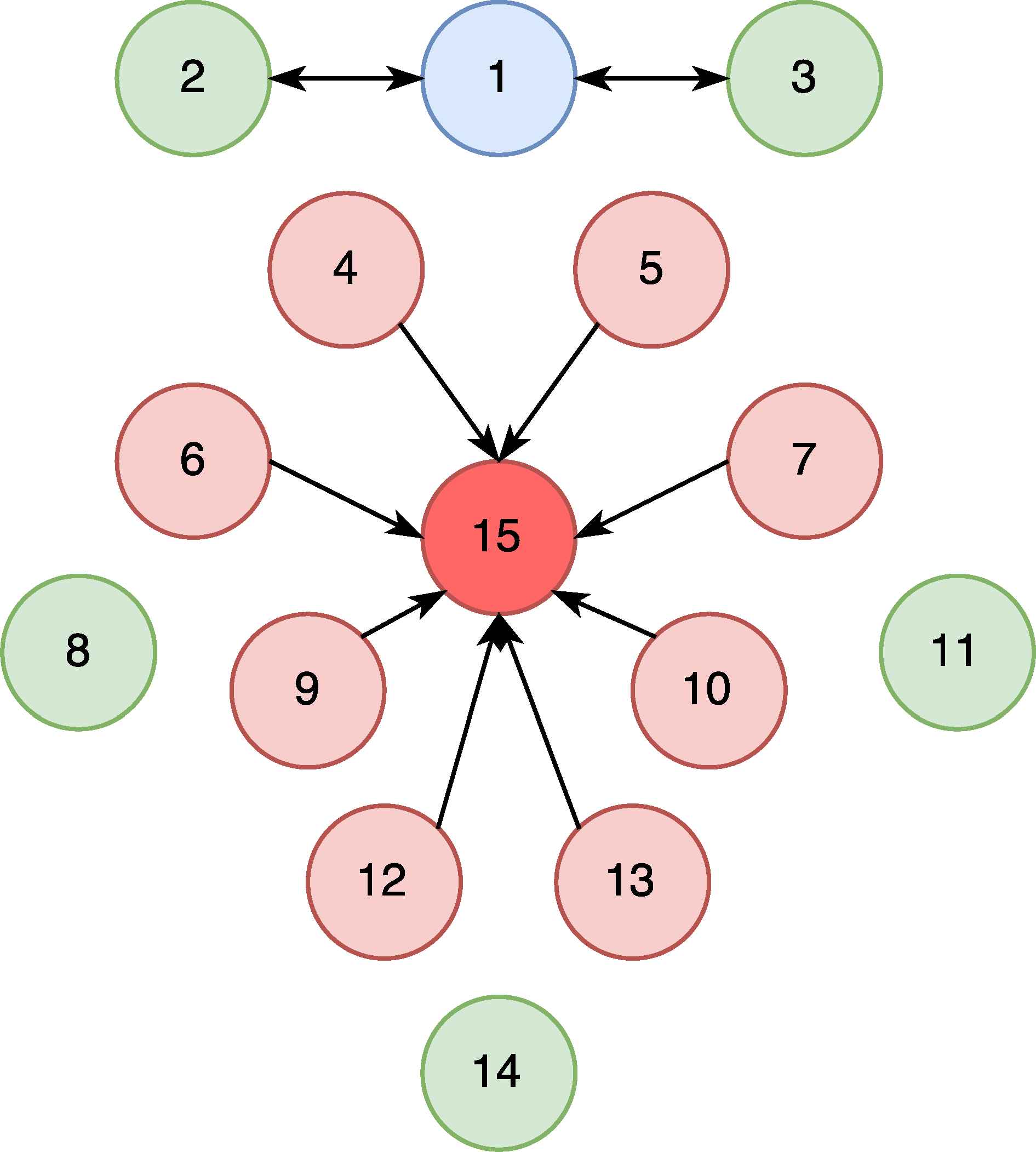
The main purpose of the HELLO message is to introduce and integrate new nodes to the network. The nodes broadcast HELLO messages with their own metrics such as signal power and ID number. All the other nodes create their own routing table to send their messages. A malicious node sends HELLO messages by DIS packets to its victims by strong signal power and suitable routing metrics, appearing like an neighbour node. The attacker node becomes the most favorable node for the victims. This attack is called the Hello-flood attack. The initialization part of this attack is depicted in Figure 6.
Before HF Attack
The malicious node, Node 15, broadcasts HELLO messages to Nodes 4-13, except Nodes 8 and 11. The victim nodes change their routing table because the malicious nodes advertise higher quality metrics. The effect of the HF attack is depicted in Figure 7.
After HF Attack
As a result of this attack, the number of transmitted packets of the malicious node increases. Accordingly, we calculate Transmission Rate (TR) (3), Transmission Average Time (TAT) (4), Transmitted Packets Counts (TPC), Total Transmission Time(TTT) and DIS features to identify this attack.
In the RPL protocol, when version numbers of nodes are changed by the root node, each node starts communication to reconstruct their own routing table. As a result, the network topology (DODAG tree) is changed. In the version number modification attack, the malicious node changes its version, then other nodes are forced to change their routing table. So that the malicious node promotes itself to take a better place in the routing table of other nodes. This can have an adverse effect on the network information security and network performance due to changed topology32.
After the attack initialization, the malicious node gets all the packets destined to the neighbour nodes. In analogy to the DR attack, we calculate Reception Rate (RR) (1), Reception Average Time (RAT) (2), Received Packets Counts (RCP), Total Reception Time (TRT), DIO and DAO packet count for detecting this attack.
3.3. Data Preprocessing and Feature Extraction
For the DR, HF and VN attacks, we have generated various attack scenarios at a wide scale number of IoT nodes, ranging from 10 up to 1000 nodes, with a different percentage (5%, 10%, 20%, etc.) of malicious nodes. As the result of the simulations, raw datasets were produced.
function array ← RAWdataset.csv Sorted array ⊳ Sorting by time Feature conversion Feature Extraction: Window Size ← 1000ms Calculate Feature values within window size Label the dataset End of the Feature Extraction End the function. |
Enrichment of IoT RAW Dataset
As explained in Section 3.1, we obtain raw data files after the simulation. However, the raw data files are not sufficient for being input to the learning algorithm because the raw dataset includes information such as source/destination nodes address and packet length, which causes noise and overfitting in learning algorithm. For these reasons, we implemented a data preprocessing and feature extraction algorithm in Python by using Pandas33 and Numpy28 libraries. These libraries perform the pre-processing operations which are necessary for easier feature extraction.
We implemented a dictionary structure to deal with a large number of nodes. We opted not to calculate global statistics over total simulated time or total packet count since this kind of calculation could adversely effect the calculation of weights of extracted features. We have divided all the simulation to time frames, or windows of 1000 ms duration. Before this process, it is necessary to sort the datasets by simulation time, because a correct sequence of packet simulation time is necessary for correct feature value calculations. The calculation of feature values is done according to the formulae provided in Section 3.2. The pseudocode of the data preprocessing and feature extraction algorithm is provided in Algorithm 1.
Raw datasets include data types which are not able to be processed by the learning algorithm, such as IP adresses. The source and destination addresses are converted from IPv6 format to Node ID. For example:
The broadcast packets are handled as follows. In a raw dataset, if the destination address is ff02::1a, that means the source node sends broadcast packets. This value is converted to 9999 to avoid any coincidence with another node:
We have also encoded the information of the packets, as shown in Table 3. DAO is used in the RPL protocol for sending out unicast destination information about to the selected parents. DIO is the most important message type in RPL. It keeps the current rank of the node, determines the best route through the base node by using specific metrics as distance or hop-count. Another message type is DIS. Nodes use DIS for getting the DIO messages. ACK is an acknowledgment message type for using to give response by nodes31. These are encoded respectively as 1, 2, 3 and 4. Other types in our datasets are Protocol Data Unit (PDU) and UDP packets which are simulated data packets.
| Info | Value |
|---|---|
| RPL Control (Destination Advertisement Object) | 1 |
| RPL Control (DODAG Information Solicitation) | 2 |
| RPL Control (DODAG Information Object) | 3 |
| ACK | 4 |
| Data Packets | 5,6,7 |
Encoding of the Packet Information Feature
As a result of feature extraction, a total of 18 candidate features are produced, which are also listed in Table 4. These values are calculated as follows. First, we calculate the Transmitted and Received Packets Counts (TPC and RCP) for each node in 1000ms in a specified time frame. Then, we divide these values to 1000ms and get Transmission Rate and Reception Rate for each node, TR (3) and RR (1) respectively, for all time frames. Duration time for each packet transmission and reception are calculated. Total Transmission Time(TTT) and Total Reception Time(TRT) are calculated by adding up duration time of each transmission and reception packet in 1000ms. Then Transmission and Reception Average Time for each node, TAT (4) and RAT (2), are calculated. The other features are about control packets; DAO, DIO and DIS. Number of transmitted control packets of each node are calculated within the windowing size, 1000 ms.
| Number | Name/Abbr. | Description |
|---|---|---|
| 1 | No. | Packet seq. nr. |
| 2 | Time | Simulation time |
| 3 | Source | Source Node IP |
| 4 | Destination | Destination Node IP |
| 5 | Length | Packet Length |
| 6 | Info | Packet Information |
| 7 | TR | Transmission Rate |
| 8 | RR | Reception Rate |
| 9 | TAT | Transmission Avg. Time |
| 10 | RAT | Reception Avg. Time |
| 11 | TPC | Transmitted Packes |
| 12 | RPC | Received Packets |
| 13 | TTT | Total Transmission Time |
| 14 | TRT | Total Reception Time |
| 15 | DAO | DAO Packets |
| 16 | DIS | DIS Packets |
| 17 | DIO | DIO Packets |
| 18 | Label | Label: Benign/Malicious |
Candidate Features as a Result of Feature Extraction
The labelling process is also important. In our datasets, since malicious nodes affect the all network activity and influence normal node communication, the traffic which includes malicious node and activity is labelled as 1 and benign traffic is labelled as 0. Then the dataset is produced by normalizing and mixing malicious and benign traffic. The normalization process will be explained in the next section.
A sample of the preprocessed dataset is shown in Table 5. The data items are selected randomly from the “VN1000” traffic data.
| Time | Src | Dst | Ln | Inf | TR | RR | TAT | RAT | TPC | RPC | TTT | TRT | DAO | DIS | DIO | Label |
|---|---|---|---|---|---|---|---|---|---|---|---|---|---|---|---|---|
| 48.45566 | 94 | 893 | 76 | 1 | 0.197 | 0.197 | 197 | 197 | 0.012 | 0.012 | 0.00006 | 0.00005 | 197 | 0 | 0 | 1 |
| 48.45569 | 389 | 339 | 76 | 1 | 0.096 | 0.096 | 96 | 96 | 0.005 | 0.005 | 0.00005 | 0.00005 | 96 | 0 | 0 | 1 |
| 48.45576 | 158 | 620 | 76 | 1 | 0.196 | 0.166 | 196 | 166 | 0.01 | 0.008 | 0.00005 | 0.00005 | 166 | 0 | 30 | 1 |
| 48.45577 | 971 | 271 | 76 | 1 | 0.22 | 0.22 | 220 | 220 | 0.008 | 0.008 | 0.00004 | 0.00004 | 220 | 0 | 0 | 1 |
| 48.45577 | 994 | 331 | 76 | 1 | 0.227 | 0.227 | 227 | 227 | 0.008 | 0.009 | 0.00004 | 0.00004 | 227 | 0 | 0 | 1 |
| 48.45578 | 354 | 894 | 76 | 1 | 0.284 | 0.128 | 284 | 128 | 0.006 | 0.006 | 0.00005 | 0.00005 | 284 | 0 | 0 | 1 |
| 48.45581 | 565 | 9999 | 97 | 3 | 0.03 | 1.7 | 30 | 1698 | 0.002 | 0.097 | 0.00007 | 0.00006 | 0 | 0 | 30 | 1 |
| 48.45583 | 808 | 792 | 76 | 1 | 0.263 | 0.189 | 263 | 189 | 0.01 | 0.006 | 0.00004 | 0.00003 | 189 | 0 | 74 | 1 |
| 48.45599 | 691 | 134 | 76 | 1 | 0.19 | 0.19 | 190 | 190 | 0.012 | 0.012 | 0.00006 | 0.00006 | 190 | 0 | 0 | 1 |
| 48.45600 | 430 | 33 | 102 | 3 | 0.171 | 0.171 | 171 | 171 | 0.013 | 0.013 | 0.00006 | 0.00006 | 0 | 0 | 171 | 1 |
Sample Dataset (Packet sequence number omitted)
After feature extraction process, the datasets include up to 26x106 data items which shows why a deep learning based methodology is needed.
3.3.1. Feature Normalization
Data resulting from different IoT routing attack scenarios have different mean and variance due to their network topology, which reduces the performance of the learning algorithm. Therefore a feature normalization process is performed. We have applied quantile transform and min-max scaling to datasets, respectively27. Quantile transformation adjusts feature value distribution to normal distribution. It aims to reduce the negative effect of marginal values. Then we scale all values in the datasets to the range 0-1 by min-max scaling. The effect of feature normalization process to features are depicted in Figures 8 and 9.
Transmission Rate before Feature Normalization Process
Transmission Rate after Feature Normalization Process
Finally all data resulting from different network topologies are concatenated to produce a dataset for an IoT routing attack type. As a result, we achieve three attack datasets, as seen in Table 1. The collection of these datasets is called IRAD. The pseudocode of our data normalization algorithm is given in Algorithm 2.
function Mixed Dataset ← Benign, Malicious Dataset Feature Normalization: Transformed Dataset ←Quantile Transform (Mixed Dataset) Min Max Scale (Transformed Dataset) End of Feature Normalization IRAD ← Mixed Datasets ⊳ concatenating the datasets End the function. |
Data Normalization Algorithm
3.3.2. Feature Selection
Feature selection is a key step in machine learning. Feature selection is generally applied to the dataset before running the machine learning algorithm, because it eliminates the irrelevant, weakly relevant features and selects the optimal subset of all features. It identifies the proper subset of all data features and makes the data serviceable. There are two main challenges; the large size of data and its inconvenient form. A dataset has two dimensions; number of instances and number of features, one or both of which could be too large. This huge volume also brings a complexity. On the other side, datasets are created from data without features or attributes. In this regard, correct modeling of the effects of the attack on the network becomes the most important step. Particularly, IRAD is produced by processing features of network packets captured from the Internet or closed network as PCAP form.
We used a combination of random decision trees (random forests), histograms and pearson coefficient correlation34 for feature selection process. We evaluated the importance of the extracted features by using a number of randomized decision trees (extra trees). Main idea of randomized decision trees is bagging, that means to adjust noisy and unbiased models to create a model in low variance. Random decision trees work as a large collection of decorrelated decision trees. Main idea of randomized decision trees is bagging, that means to adjust noisy and unbiased models to create a model in low variance. Random decision trees work as a large collection of decorrelated decision trees. In brief, randomized decision trees create different decision trees and extract importance of features by comparing the created trees35. For this purpose we utilized the RandomForestClassifier function of the sklearn library with the number of estimators set at 100. Subsequently we determine the efficient features. If the importance is high, a feature dilutes the effect of others and it may cause over-fitting at the learning process.
Different feature selection methods should be applied for different type of attacks, since feature importance rates are different based on dataset content. For the DR attack, importance rates are listed in Table 6. As clearly seen in this Table, some features cause bias over other features. The rates in the table are initially measured importance rates. First, the most significant feature is dropped, to avoid over-fitting, and the least significant feature is dropped, to avoid under-fitting. The importance rates are recalculated and the process is re-iterated, the learning algorithm is executed and results are evaluated. The process continues until the best set of features are determined.
| Feature | Importance | Selected |
|---|---|---|
| No. | 0.0186 | No |
| Time | 0.0183 | No |
| Source | 0.8382 | No |
| Dest. | 0.0119 | No |
| Length | 0.0039 | No |
| Info | 0.0047 | No |
| TR | 0.0113 | Yes |
| RR | 0.0084 | Yes |
| TAT | 0.0087 | Yes |
| RAT | 0.0068 | Yes |
| TPC | 0.0230 | Yes |
| RPC | 0.0073 | Yes |
| TTT | 0.0124 | Yes |
| TRT | 0.0083 | Yes |
| DAO | 0.0091 | Yes |
| DIS | 0.0003 | No |
| DIO | 0.0101 | Yes |
Feature Importance of DR Attack
Feature importance rates for the selected features of the DR attack are shown in Figure 10, as an example. Here, X axis represents abbreviation of selected features. Y axis represents the importance rate of features.
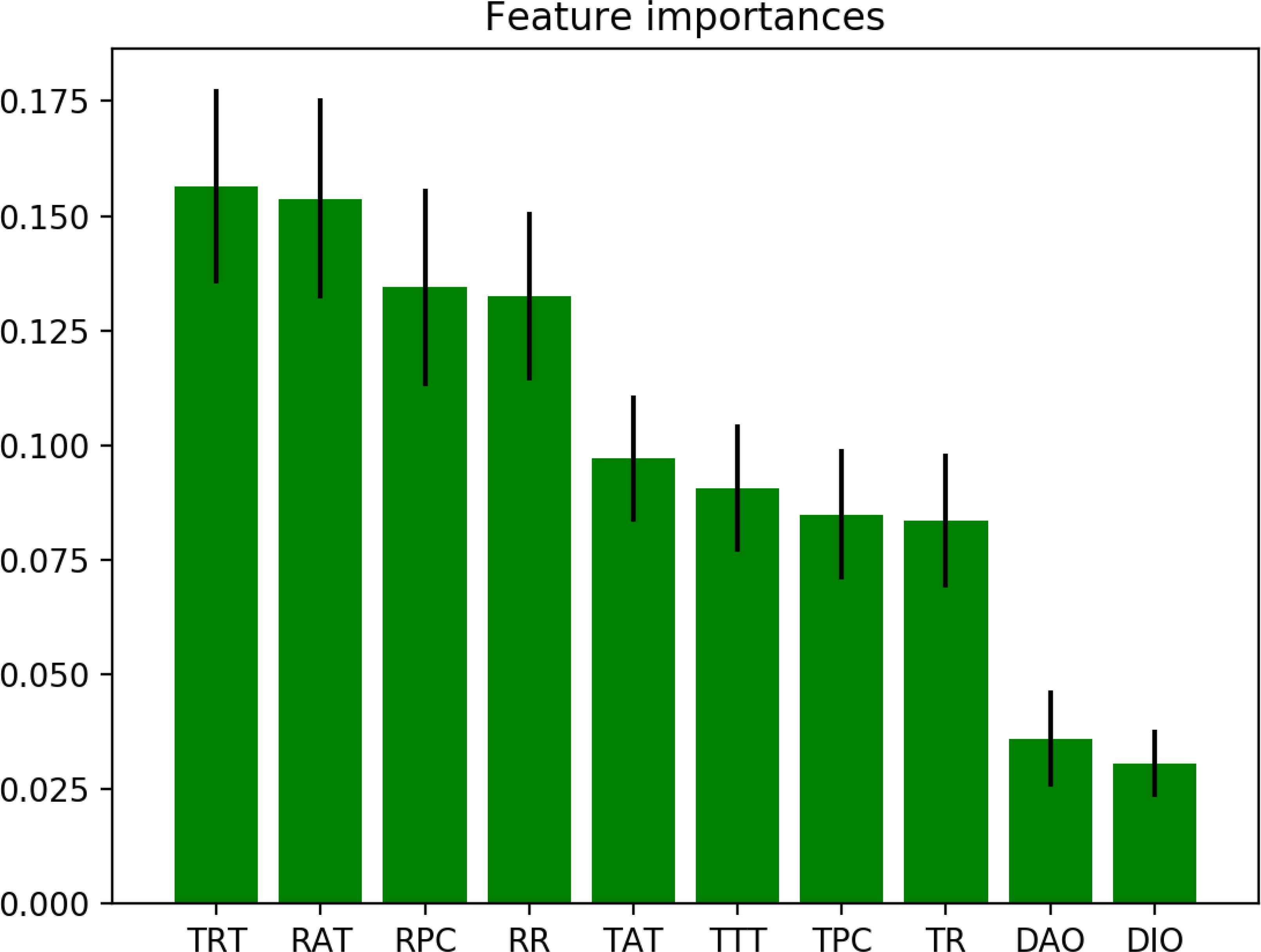
Feature Importance for DR Attack after Feature Selection
We also extracted dataset histograms to observe differences 0 and 1 within each feature. If the line corresponding to the 0 label is significantly different from the line of the 1 label in a feature, and it follows the histogram distribution for 0 labels, it is a significant feature for the learning algorithm. Otherwise, the label distributions are close to random noise, hence the feature is insignificant and the learning algorithm is not able to use the feature effectively.
Two sample histograms of a significant and an insignificant feature from the VN dataset are shown in Figure 11 and 12, respectively. The significant feature sample belongs to the Transmission Rate feature and the insignificant feature sample belongs to the Packet Length feature.

Transmission Rate Histogram of VN dataset
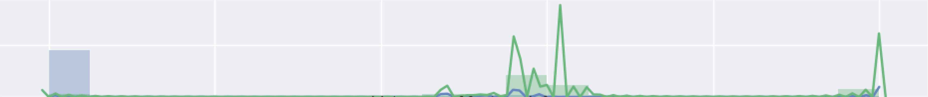
Packet Length Histogram of VN dataset
We also evaluated the Pearson coefficient of our datasets to measure correlation between features. The pearson coefficient correlation is used to understand the level of dependency between the features and the data. Guyon et al. 34 asserts that the Pearson coefficient correlation is appropriate for binary classification problems. Additionally, using Pearson coefficient correlation gives some information about linearity and nonlinearity of the dataset. Pearson coefficient correlation has a value within 1 and -1. 1 means total positive linear correlation, -1 means total negative linear correlation and 0 means nonlinear correlation. The basic formula for calculation of Pearson coefficient correlation is shown in Equation 7. In this formula, ρx,y represents Pearson coefficient correlation, cov is the covariance, σx and σx are standard deviations of x and y, respectively.
Additionally, visualization of the Pearson rate coefficient also helps in a deeper understanding feature-label correlations. As an example, Pearson rate of the TTT feature is depicted in Figure 13.
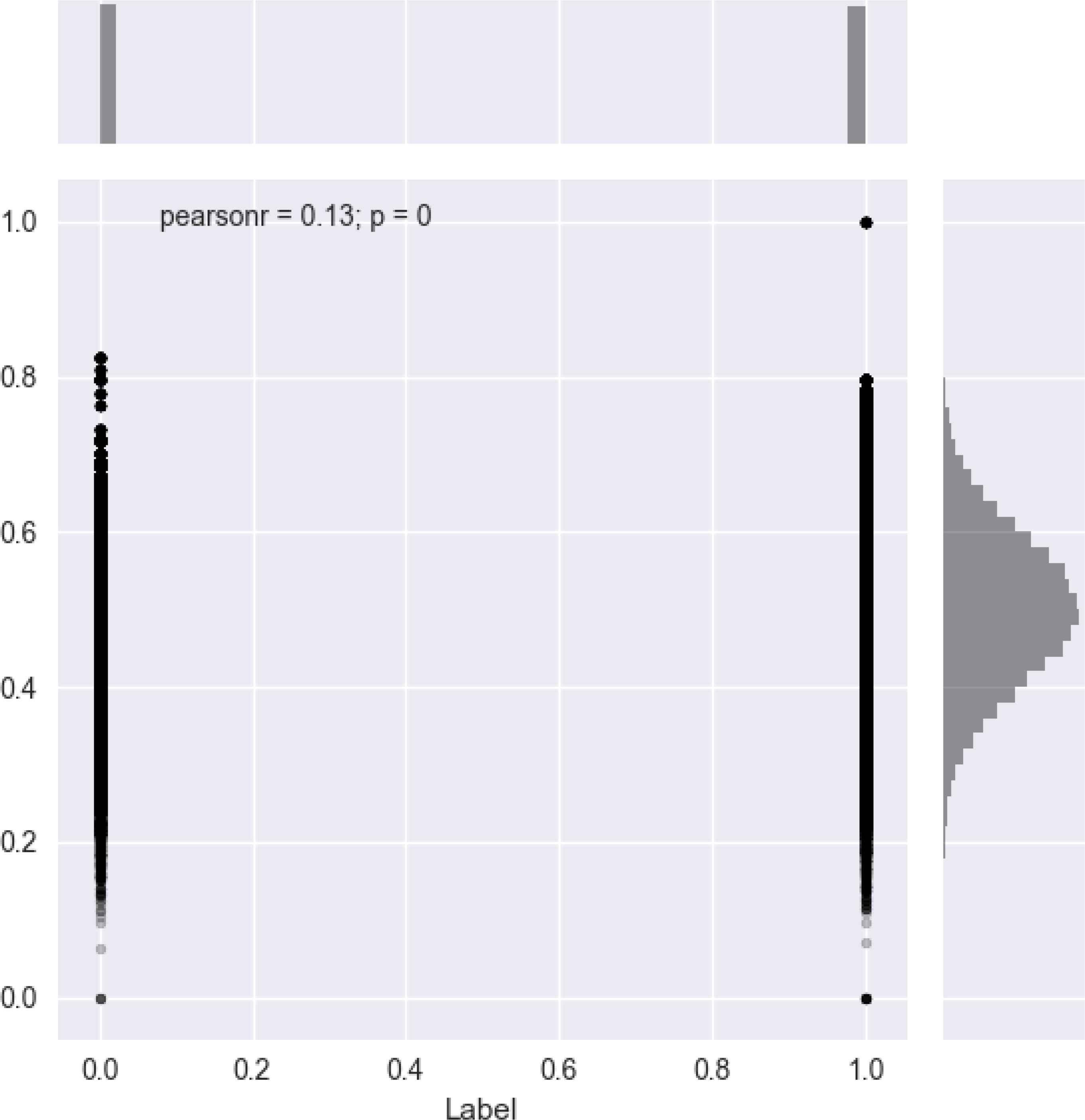
Pearson coefficient of TTT feature
Feature normalization is a pre-processing method for scaling all values of each feature into a certain range. It makes the data smoother and cleans the bias from data, ensuring high accuracy rate36. However we apply the feature normalization process to our dataset by taking all value into certain range.
Since the dataset is obtained through simulation, we have conducted additional experiments using other classifiers in order to baseline our model. Our aim is to compare our method to shallow learning and to establish a baseline for the applicability of our dataset to the proposed problem. The results are given in Table 7.
| Dataset | Score | MLP | Naive Bayes | |||
|---|---|---|---|---|---|---|
| Relu | Identity | Logistic | Tanh | |||
| VN | Precision | 0.77 | 0.68 | 0.76 | 0.77 | 0.62 |
| Recall | 0.77 | 0.68 | 0.74 | 0.76 | 0.62 | |
| F1 | 0.77 | 0.68 | 0.74 | 0.76 | 0.62 | |
| AUC | 0.75 | 0.67 | 0.75 | 0.76 | 0.61 | |
| HF | Precision | 0.97 | 0.94 | 0.97 | 0.97 | 0.89 |
| Recall | 0.97 | 0.93 | 0.97 | 0.97 | 0.89 | |
| F1 | 0.97 | 0.93 | 0.97 | 0.97 | 0.89 | |
| AUC | 0.97 | 0.93 | 0.96 | 0.97 | 0.88 | |
| DR | Precision | 0.72 | 0.56 | 0.70 | 0.71 | 0.55 |
| Recall | 0.72 | 0.59 | 0.70 | 0.72 | 0.59 | |
| F1 | 0.72 | 0.50 | 0.70 | 0.71 | 0.53 | |
| AUC | 0.70 | 0.51 | 0.68 | 0.70 | 0.52 | |
Experiments with Shallow Classifiers
We conducted analyses using the MLP (Multi-Layer Perceptron) and Naive Bayes classifiers. MLP is a feed-forward ANN with at least three layers of nodes. For the MLP, a one hidden layer multi-layer perceptron is used, using different activation functions. Naive Bayes is a simple probabilistic classifier that is based on Bayes theorem and it assumes naive independence between features. Based on these results we can conclude that the shallow classifiers do not perform well for our problem.
3.4. Deep Learning Algorithm
Deep learning (DL), is a ML hierarchical representation, is based on Artificial Neural Networks (ANN). Difference between ’old school’ ANN and DL is that DL involves many hidden layers37. With the advent of GPU computing, the training durations of DL networks are reduced, which has led to a mainstream adoption of DL38,39. In DL, some advance training methods, such as Deep Belief Network(DBN)38 or Convolutional Neural Network(CNN)40, make effective solutions when applied to specific problem. DL also has the capability to extract additional features itself, based on the initial set of features provided to the algorithm, which enables the learning process to be more accurate.
DL is not a distinctive algorithm or another branch of AI. It can be used in supervised, unsupervised and reinforcement learning. Another advantage is that DL is built on an easily modifiable architecture which enables to create a solution to specific problem. For example, reinforcement learning (RL) differs from supervised and unsupervised learning such that the actions are evaluated according to their outcomes, i.e. RL learns the sequences of actions that will lead to the achievement of a goal or maximization of an objective function.
DL networks are usually trained by using back-propagation algorithm that helps to find error gradient of loss function which is required due to gradient descent algorithm. Back-propagation finds the error gradient faster than previous algorithms41.This formula is presented in Equation 9. Here, Wij denotes the connection weight from neuron i in layer m to neuron j in layer m + 1 and
This formula enables to adjust the weights of each layer as a derivation of the previous layer to enhance the accuracy. The problem is missing weight adjustment due to derivative transactions. It’s called vanishing gradient problem that limits depth of NN. For this reason, when this formula is used, a single hidden layer is preferred rather than multi hidden layers. There is another function as a solution of the vanishing gradient problem called Rectified Linear Unit (ReLU). The mathematical equation is shown at 10.
If input is less then zero, output equals zero, otherwise input bigger then zero, output equals input. So it, has a non-vanishing derivative and is usually preferred for the back-propagation optimization problem. For binary classification, ReLU function is more suitable and we use it in the hidden layers as the activation function.
In this study, Keras is utilized as the deep learning framework that ensures many advantages. First, Keras is integrated into the vast Python data science ecosystem. Second, Keras has a well documented user manual and many examples. After that, Keras enables to build complex neural networks easily. Last but not least, TensorFlow, one of the most popular machine learning frameworks, is accessible with Keras.
In the implementation of the learning algorithm based on deep learning, we used first the dataset is shuffled, to improve deep model performance and avoid overfitting. Before building the neural layers, the pre-processed dataset is split into two parts. The first part, X, is the part of the dataset which excludes the label feature. The second part, Y is the other part of the dataset which includes the labels. Accordingly, Y is the part what makes this algorithm a supervised learning algorithm. After the splitting step, X and Y are evaluated through the Randomized Decision Trees method to calculate feature importance rates. This process is fully automatized, i.e. the features causing under-fitting and over-fitting are dropped. For creating the deep neural network model, we used the sequential model. Mean squared error (MSE) is used as the loss function. Since we have a binary classification problem, MSE is a suitable choice. The selected optimizer is the AdaDelta43 algorithm. This algorithm has the advantages that only first order information is necessary for adapting over time, and has a minimal computational overhead beyond the Stochastic Gradient Descent (SGD) algorithm. In our experiments we found that this optimizer performs the best for our problem. Cross validation is often not used for evaluating deep learning models because of the greater computational expense. We have applied shuffling and used a random subset of the training data as a hold-out for validation purposes. Test-train split is performed as follows: X and Y are split into two parts; X_train, X_test, Y_train and Y_test. X_train and Y_train are used in the training section. X_test and Y_test are used to evaluate the performance of the trained model. Before the training starts, dataset split is applied once more again at a rate of 0.1 to produce a Validation dataset. The Validation dataset is used to calculate the performance of the trained model. After the training process, we save the created model and weights as a JSON file. Finally, we test our model for routing attacks detection by applying the model.predict function on other datasets.
We use the Sigmoid function as the activation function for output layer. This function is also known as the logistic function, it has a characteristic as ’S’ curve and the mathematical representation is shown at 11. Other functions, such as Step and Linear activation functions, are not suitable for our problem, since they exhibit non-linear characteristics. The other two candidate activation functions, Softmax and Tanh function have been evaluated by experimentation, however they have yielded low accuracy rates; 35.3% and 35.8%, respectively. The accuracy of model has reached up to 99.5% when we use Sigmoid function in the output layer.
Our neural network architecture consists of 7 layers. The first layer is the Input Layer, that has 10 neurons. The number of input layers should be equal to the number of features (columns) in dataset. The last layer is the output layer that has just a single neuron. This is called the Regression Mode. Our neural network has 5 hidden layers. The first and fifth layers have 50 neurons. The second and fourth layers have 100 neurons. The third layer has 300 neurons. The neural network model for DR and VN attacks are shown in Figure 14. The HF neural network model is similar except that the input layer consists of 5 neurons.
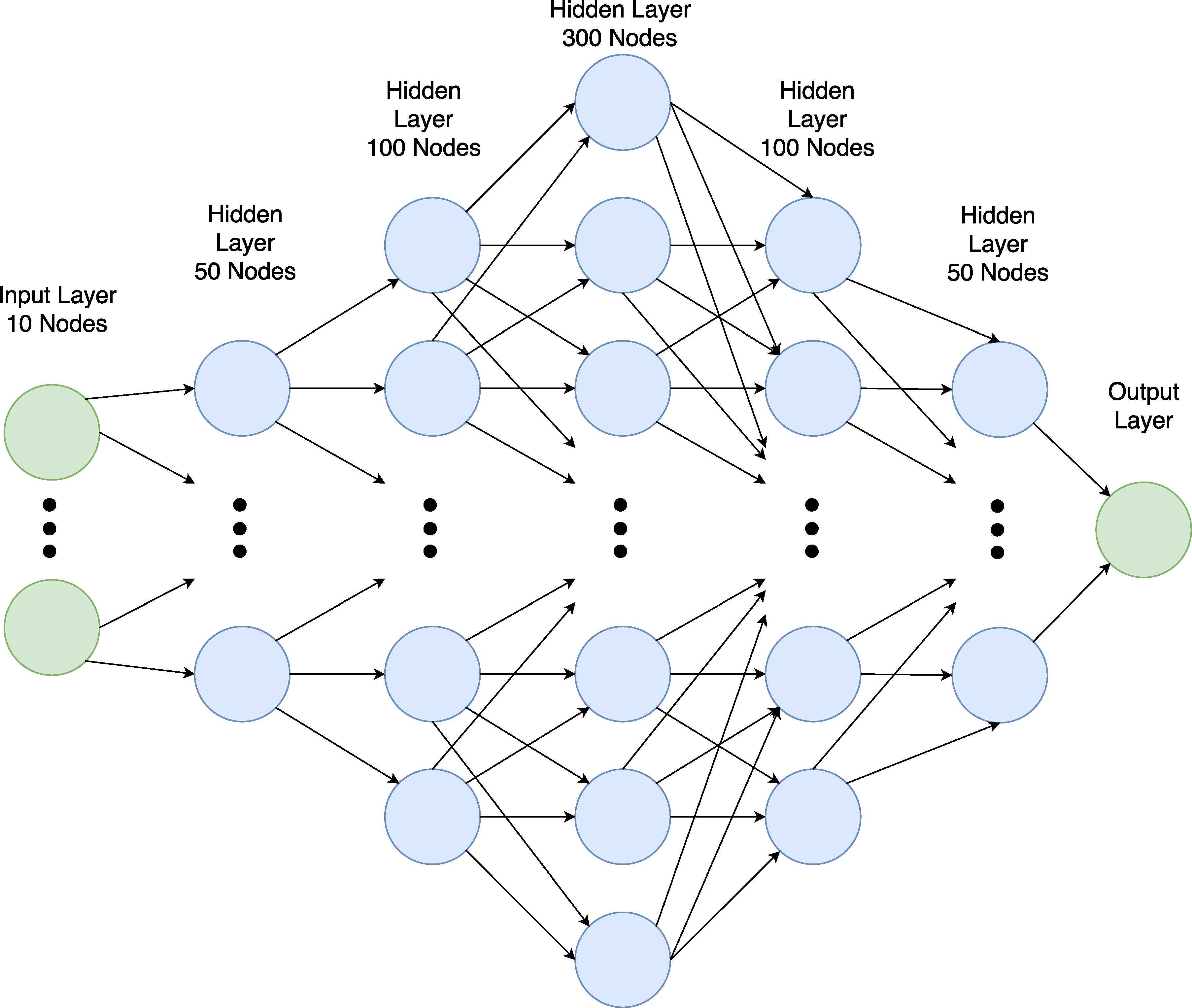
Neural Network Model for DR and VN Attacks
We applied best practice and experimentation while creating neural network architecture. Recent studies for finding proper network sizes and architectures44 report that trial-and-error approach is inevitable for complex models. Similarly, in our study the number of neuron layers and neuron counts were obtained by experimentation. In particular we adopted the so-called backward trial-and-error approach, where a large number of neurons are initially used. The network is trained and tested. When the network exhibits overfitting, the number of hidden neurons are gradually decreased. This process is repeated until satisfactory performance is obtained while avoiding overfitting.
The pseudocode of our deep learning algorithm is given in Algorithm 3.
|
Deep Learning Algorithm
In the training process, we also avoid sharp increases by applying dropout and regularization. Such sharp increases imply that the learning function gets stuck in local minima. With experimentation, we have found that the best dropout rate is 10%. The dropout technique helps deal with the over-fitting problem. When applying dropout, some nodes located in the hidden layers are removed randomly at each iteration (epoch). Additionally we also apply bias regularization to diminish non-linearity of training by limiting the peak results. Therefore, the coefficients of our deep layers are much smaller, which helps the training process to reach global minimum in the loss function.
3.5. Performance Metrics and Class Imbalance
The key point of attack detection is to achieve high effectiveness which is calculated by using performance metrics. All performance measurements are based on confusion matrix which shown in Table 8.
| Predicted Positive | Predicted Negative | |
|---|---|---|
| Real Positive | True Positive (TP) | False Negative (FN) |
| Real Negative | False Positive (FP) | True Negative (TN) |
Confusion Matrix
If a system says there is an attack and that is true, this prediction is a True Positive (TP), also called positive class accuracy or sensitivity. If the system says there is no attack and and that is true, this prediction name as a True Negative (TN), also called negative class accuracy or specificity. If the system indicates an attack and but that is false, this prediction is a False Positive (FP). If the system does not indicate an attack but that is false, this prediction name as a False Negative (FN). High TP and TN (low FP and FN) prediction rates are acceptable and desirable. Then the accuracy is calculated as follows.
Another important performance metrics are precision and recall. Precision and recall calculations are formalized as Equations 13 and 14, respectively. F1-score is another widely used performance metric, which is a function of precision and recall. F1-score calculation is presented at Equation 15.
However our dataset has imbalanced classes due to the our problem. The problem of imbalanced classes occurs in various applications, such as bioinformatics, e-business, information and national security.45 In anomaly detection cases, the benign activities are much more than the anomalies. We also produced our dataset like that, as shown in Table 1 in Section 1. Number of malicious nodes are quite few than number of benign nodes. However, we realized that the malicious nodes harm all activities of the network. So we labelled all the network, which include malicious node(s), activity as 1 (being affected). That is explained in Section 3.3. Then we generated benign networks that have same topology with the malicious. After combining the malicious data sets and benign datasets, we produced IoT Routing Attack Dataset, three different dataset for three different attacks to attack detection.
The mentioned performance metrics are not preferred to calculate performance of imbalanced dataset. Because, they can produce misleading results for highly imbalanced dataset. For example, assume that, we have a test dataset that has 100 packet which include just 1 malicious packet. If the model always predicts benign, accuracy will be 99%. The model seems very well for attack detection. Otherwise, if the model always predicts malicious, recall will be 100%. The model detects the malicious activity, but in the other hand, it always rises the alarm even if there is no malicious activity.46
Two different metrics are used to deal with imbalanced dataset. First one is sensitivity (or named True Positive Rate (TPR), positive class accuracy) and it is same with recall. Second one is specificity (or named True Negative Rate (TNR), negative class accuracy).45
These metrics are used to calculate the area under the curve (AUC) and a receiver operating characteristic (ROC). If the AUC-ROC is bigger than 0.5, it means that the model is better than random guessing.47
4. Results and Analysis
We created three datasets that are Decreased Rank (DR) Attack Dataset, Hello-Flood (HF) Attack Dataset and Version Number (VN) Attack Dataset. They consist both of attack and benign activities. The number of values what they include and the size of attack dataset files are listed in Table 9.
| Number of Values | Size (Gb) | |
|---|---|---|
| DR Attack Dataset | 49,873,385 | 0.58 |
| HF Attack Dataset | 64,179,435 | 0.75 |
| VN Attack Dataset | 22,868,210 | 0.27 |
Datasets with Numbers
After the dataset generation, we created an IoT dataset and named it IRAD (IoT Routing Attack Dataset) which contains up to 1000 IoT nodes and three attacks. Various scenarios have been reflected in the dataset, with different ratios of benign and malicious nodes and total node counts. Available datasets in the network attack detection area have limited applicability to the IoT domain, due to different nature (such as ad-hoc communication, wireless protocols) of IoT networks. We also compared IRAD with other similar datasets, UNSW-NB1548 and KDDCUP9924, in Table 12. The other datasets have more attack types and therefore more features. IRAD is specific to IoT, therefore it does not include generic attack types and as a result, it has less attack types than the compared datasets. We aim to introduce new IoT attack types to the IRAD dataset as our future work. At the moment, the feature set included in IRAD is more closely related to IoT routing attacks. We also plan to extend the feature set with different types of attacks, such as impersonation attacks.
Our second contribution is an attack detection neural network model based on deep learning. Starting with the same candidate features and an initial neural network model, the feature selection and deep learning process results with a specific IoT attack detection model for each routing attack. Since we have obtained high precision, recall, F1 and AUC test scores, we have shown that the obtained models are generalizable for different network topologies and sizes. The training performance of these models (Training Accuracy, Training Loss) are listed in Table 10.
| Model | Accuracy | Loss | AUC |
|---|---|---|---|
| DR Model | 94.9% | 5% | 89.6 |
| HF Model | 99.5% | 0.8% | 92.2 |
| VN Model | 95.2% | 4.1% | 90.3 |
Training Performances
The training accuracy and loss of the HF Model, as well as the prediction F1-scores are better than the other two models, since the Hello-flood attack affects less network parameters than the other two attacks. Accordingly, the best performance for the HF attack is obtained when the detection model is trained with 5 features, while the DR and VN attacks are trained with 10 features, as explained in Section 3.3.2. The performance of the DR and VN models are also high, with 0.94 and 0.95 F1-scores. However, one should take into account that, for the performance of attack detection models, the precision and recall for the positive outcome is more important. The reasoning is that, it is more acceptable to generate a false alarm than to miss an attack. From this point of view, DR and VN models also perform well, with a score equal or more than 0.95 for precision, recall and F1-scores.
We tested our deep learning based attack detection models with data produced by multiple simulation scenarios to ensure the fidelity of the models. In addition to the scenarios included in the IRAD dataset, we conducted tests on additional scenarios with different number of nodes and different network topology in addition to those included in the IRAD dataset listed in Table 1. The additional scenarios include, 200, 400, 750 and 1000 nodes with different malicious/benign node and traffic ratios. The performance figures are an average of all tests.
4.1. Decreased Rank Attack
As explained above, we tested our deep learning based DR Model with multiple scenarios with varying malicious/benign node ratios. The figures given are an average of all tests. The performance metrics are listed in Table 11.
| Precision | Recall | F1 Score | |
|---|---|---|---|
| 0 | 0.94 | 0.93 | 0.93 |
| 1 | 0.96 | 0.98 | 0.95 |
| Average | 0.95 | 0.96 | 0.94 |
Prediction Performance of DR Model
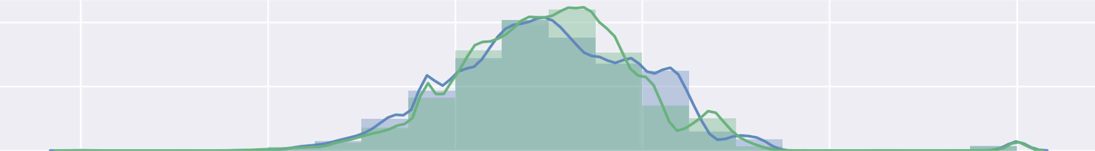
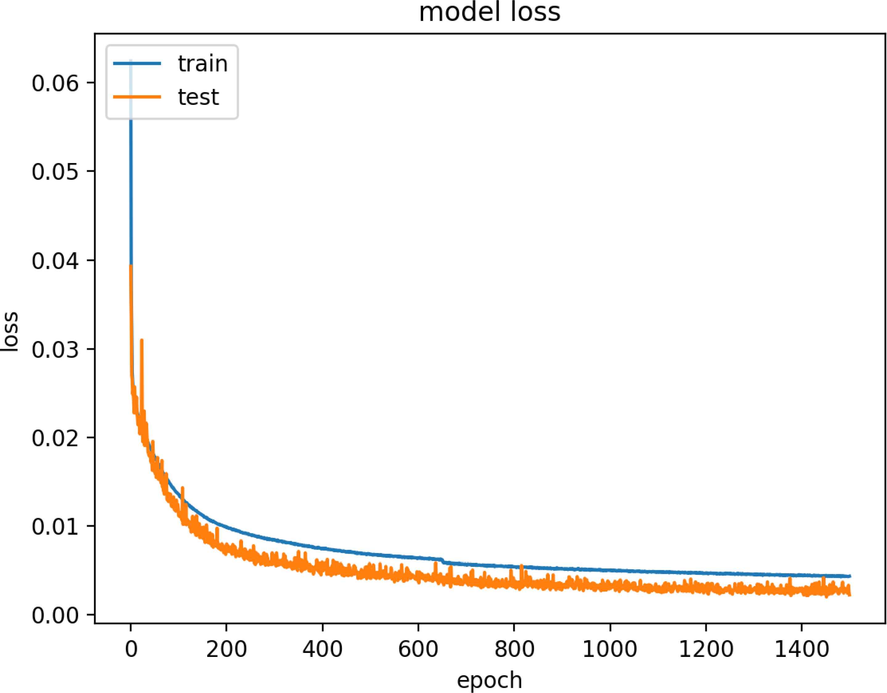
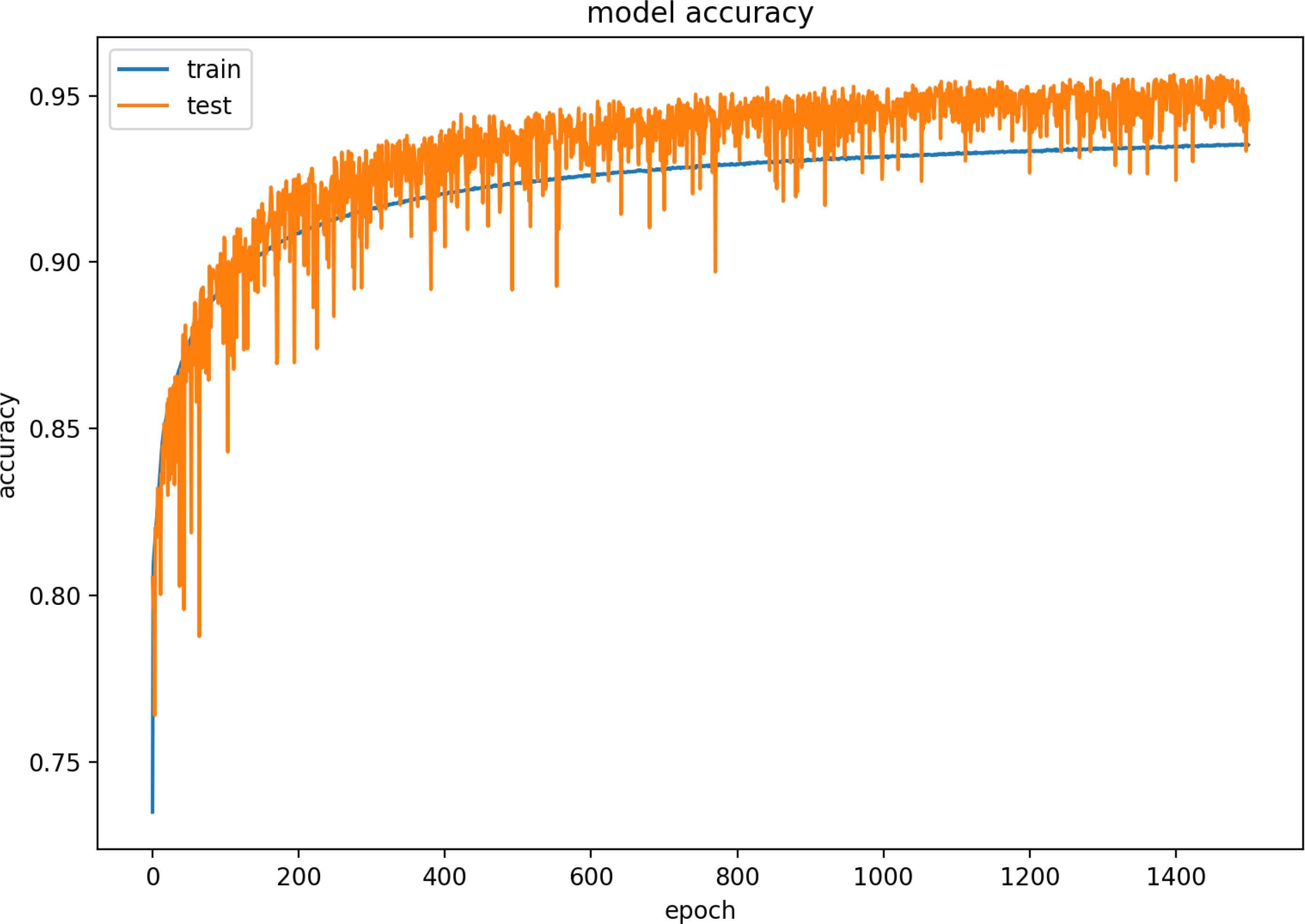
Figure 15 and 16 are model training graphs of DR Model.
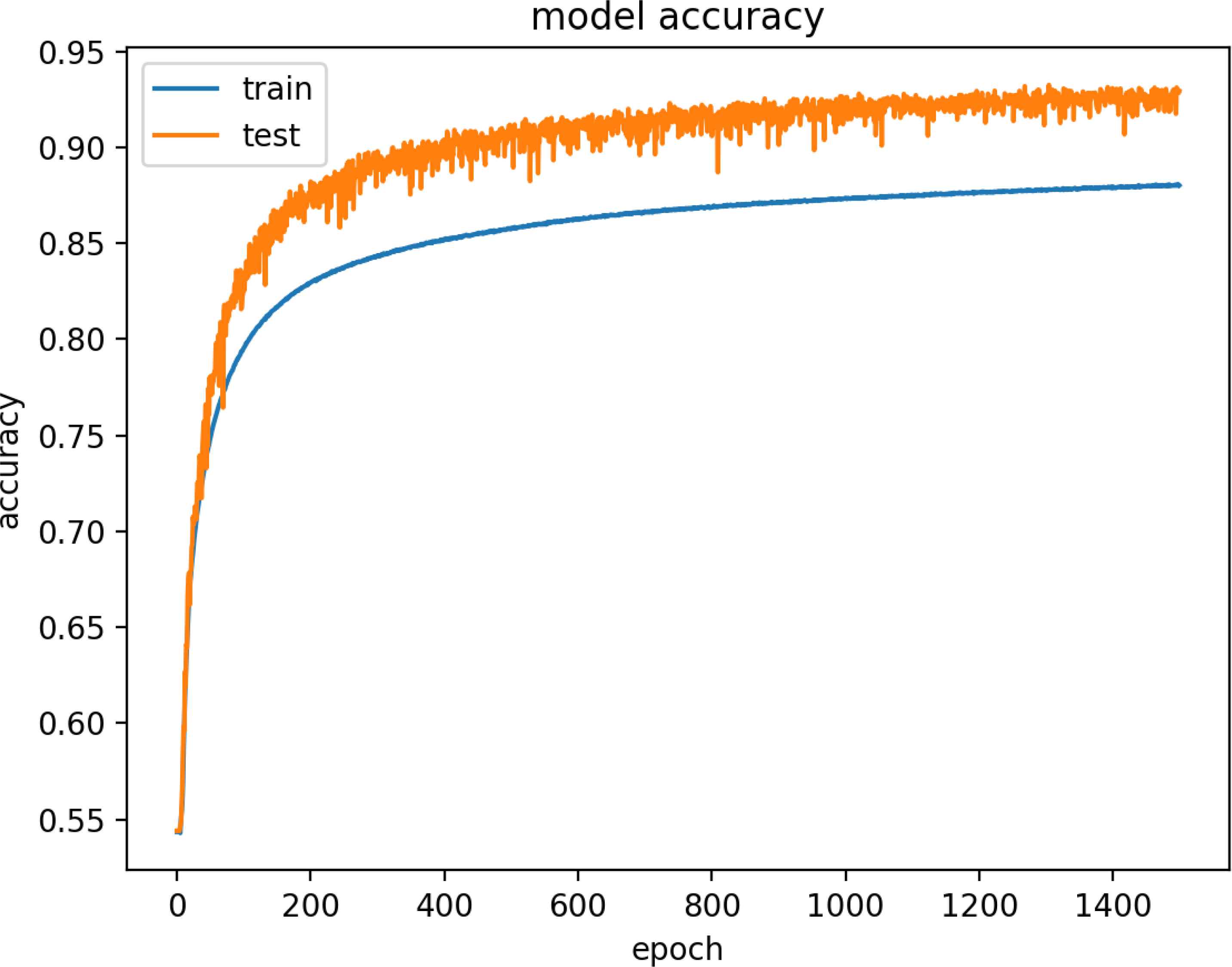
Model Accuracy of DR Dataset
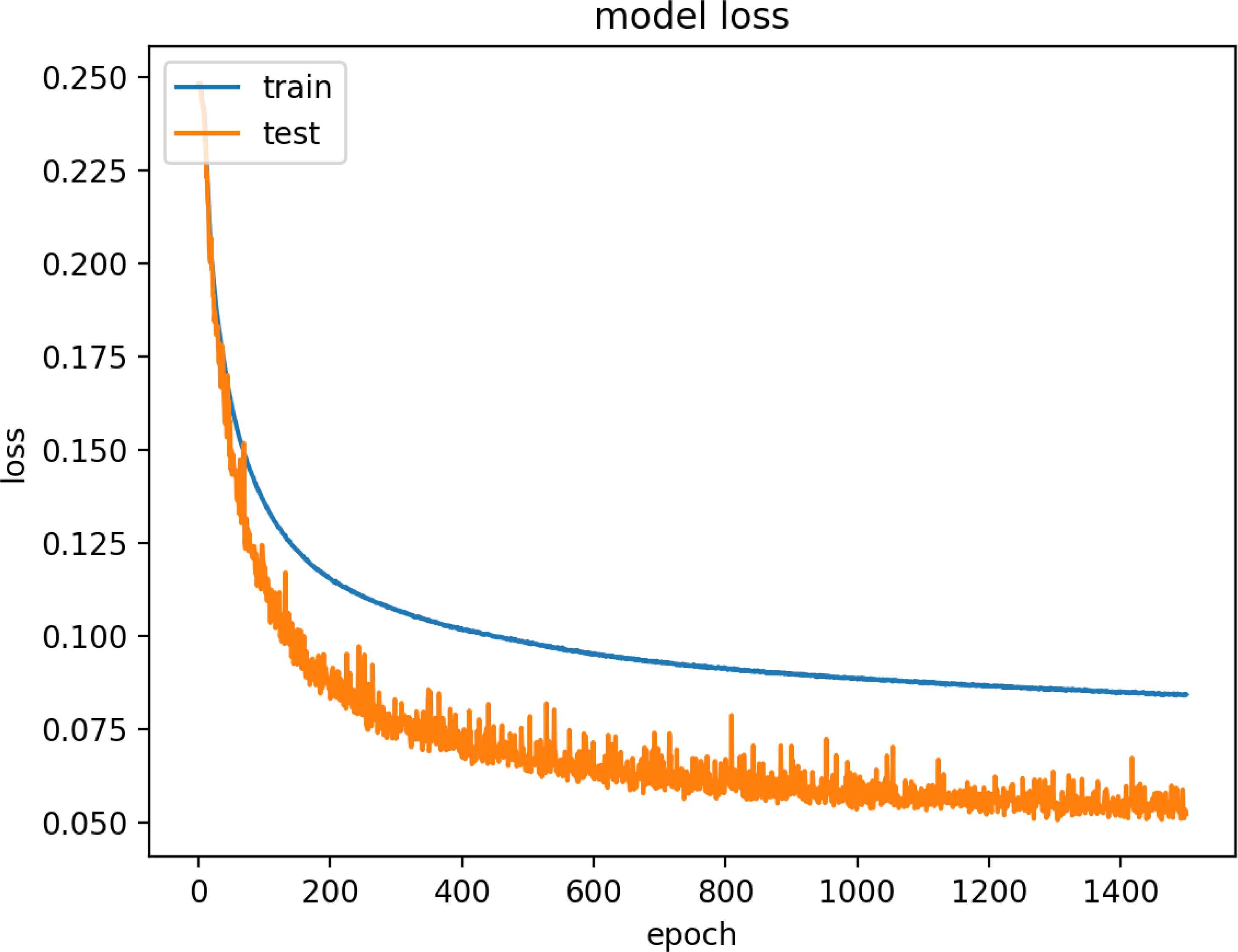
Model Loss of DR Dataset
| Parameters | UNSW-NB15 | KDDCUP99 | IRAD |
|---|---|---|---|
| Simulation | Yes | Yes | Yes |
| Attack Types | 9 | 4 | 3 |
| Number of Networks | 3 | 2 | 16 |
| Data Type | Pcap files | 3 types (tcpdump, BSM and dump files) | PCAP files |
| Feature Extraction | Argus, Bro-IDS and new tools | Bro-IDS tool | Own Implementation |
| Extracted Features | 49 | 42 | 18 |
| Distinct IP addresses | 45 | 11 | 4520 |
A Comparison of Datasets
4.2. Hello Flood Attack
Similarly, the performance metrics for the HF Model are listed in Table 13.
| Precision | Recall | F1 Score | |
|---|---|---|---|
| 0 | 0.97 | 0.98 | 0.99 |
| 1 | 0.98 | 0.96 | 0.98 |
| Average | 0.98 | 0.97 | 0.98 |
Prediction Performance of HF Model
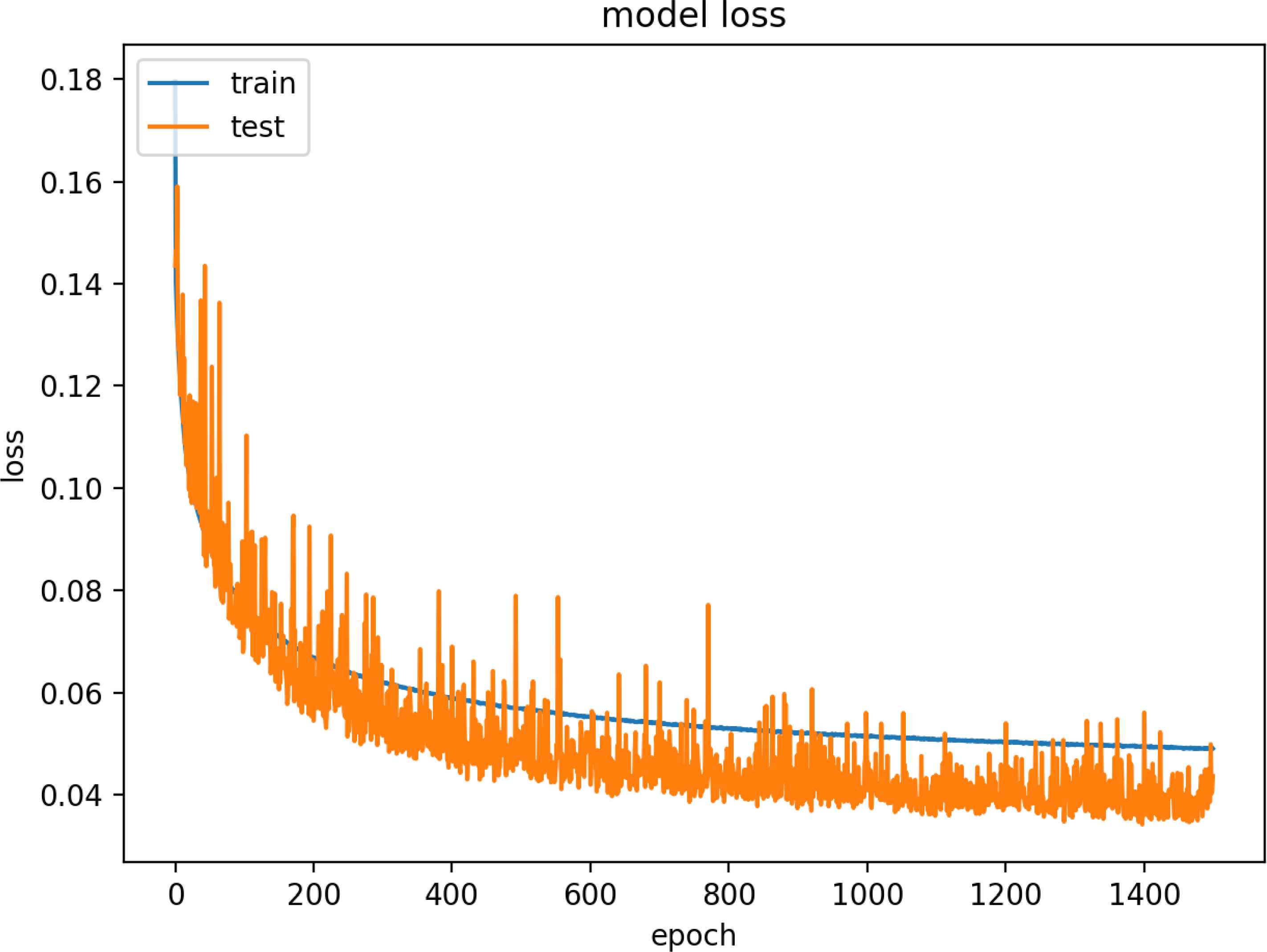
Figure 17 and 18 are model training graphs of the HF Model.
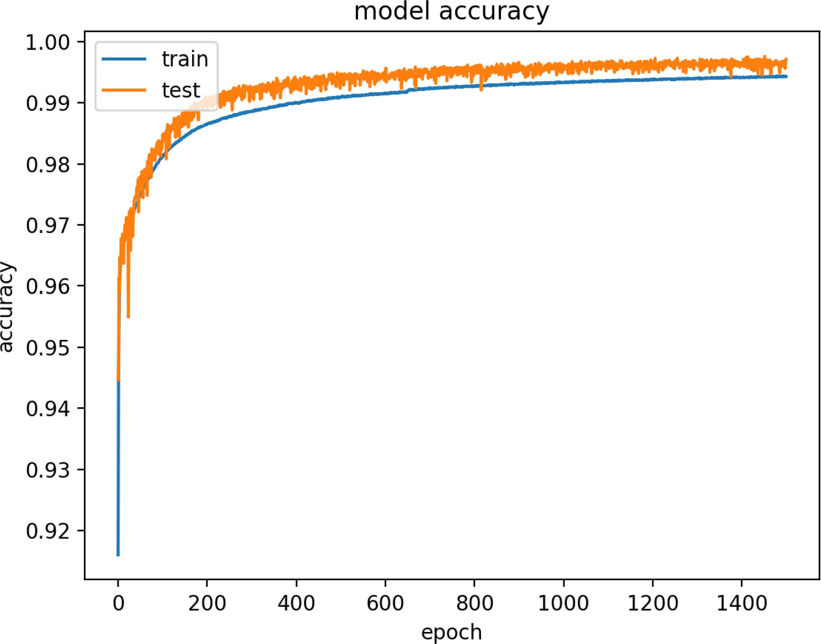
Model Accuracy of HF Dataset
Model Loss of HF Dataset
4.3. Version Number Modification Attack
Similarly, the performance metrics for the VN Model are listed in Table 14.
| Precision | Recall | F1 Score | |
|---|---|---|---|
| 0 | 0.94 | 0.93 | 0.93 |
| 1 | 0.95 | 0.95 | 0.95 |
| Average | 0.94 | 0.94 | 0.95 |
Performance of VN Model
Figure 19 and 20 are model training graphs of the VN Model.
Model Accuracy of VN Dataset
Model Loss of VN Dataset
The F1-Score performance and AUC test scores of these models are summarized in Table 15. The high performance scores indicated our attack detection models are generalizable and scalable.
| Model Name | F1-Score | AUC |
|---|---|---|
| Decreased Rank Model | 94.7% | 94.2 |
| Hello Flood Model | 99% | 98.1 |
| Version Number Model | 95% | 94.7 |
Overall Performance of the Models
5. Discussion and Conclusions
This study is a proof of concept towards application of deep learning for IoT security. Our study presents an approach which can detect routing attacks based on Big Data with high scalability and high generalization. The routing attacks (decreased rank attack, hello-flood attack and version number attack) are successfully detected by our proposed attack detection models. This work also fills an important gap for routing attack detection in IoT systems.
The biggest issue in this area is the lack of datasets and the quality of available data. Our attack datasets are produced by simulation, using real sensor code and RPL protocol implementation of Contiki-RPL. The IRAD datasets include up to 64.2 million values, which is a realistic scale for a real life IoT system. Additionally, we constructed deep neural network models trained with the IRAD datasets with high accuracy, precision and recall rates. We have obtained performance figures up to 99%, based on the F1-Score and AUC test score.
As future work, we plan to introduce additional attack types to IRAD. The dataset has three routing attacks; decreased rank (DR) attack, hello flood (HF) attack and version number modification (VN) attacks. We plan to diversify the scenarios that have different rate of malicious and normal nodes, as well as larger number of nodes.
We also aim to increase the model prediction performance of the current models and evaluate their performance on more routing attack types. For this purpose, we are investigating additional features to create a single model that could be used to detect multiple types of attacks.
References
Cite this article
TY  - JOUR
AU  - Furkan Yusuf YAVUZ
AU  - Devrim ÜNAL
AU  - Ensar GÜL
PY  - 2018
DA  - 2018/11/01
TI  - Deep Learning for Detection of Routing Attacks in the Internet of Things
JO  - International Journal of Computational Intelligence Systems
SP  - 39
EP  - 58
VL  - 12
IS  - 1
SN  - 1875-6883
UR  - https://doi.org/10.2991/ijcis.2018.25905181
DO  - 10.2991/ijcis.2018.25905181
ID  - YAVUZ2018
ER  -