
Evolutionary computation for optimal knots allocation in smoothing splines of one or two variables
Email:hasan@correo.ugr.es
- DOI
- 10.2991/ijcis.11.1.96How to use a DOI?
- Keywords
- Approximation; Smoothing; Knots allocation; Bi-cubic splines
- Abstract
Curve and surface fitting are important and attractive problems in many applied domains, from CAD techniques to geological prospections. Different methodologies have been developed to find a curve or a surface that best describes some 2D or 3D data, or just to approximate some function of one or several variables. In this paper, a new methodology is presented for optimal knots’ placement when approximating functions of one or two variables. When approximating, or fitting, a surface to a given data set inside a rectangle using B-splines, the main idea is to use an appropriate multi-objective genetic algorithm to optimize both the number of random knots and their optimal placement both in the x and y intervals, defining the corresponding rectangle. In any case, we will use cubic B-splines in one variable and a tensor product procedure to construct the corresponding bicubic B-spline basis functions in two variables. The proposed methodology has been tested both for functions of one or two independent variables, in order to evaluate the performance and possible issues of the procedure.
- Copyright
- © 2018, the Authors. Published by Atlantis Press.
- Open Access
- This is an open access article under the CC BY-NC license (http://creativecommons.org/licences/by-nc/4.0/).
1. Introduction
Function approximation, and curve/surface fitting to data, are major and important problems in many applied technical and scientific fields: as in CAD design, virtual reality and computer animation, data visualization of geological and medical imaging, artificial vision or scientific computing in general 10, 16.On the other hand, there are several different methodologies that have been used for selecting knots for best approximating or fitting curves/surfaces to data using B-splines. For instance, the methodology in 3 uses a least squares fitting method with B-spline surfaces, depending on a sensitive parametrization, in connection with a uniform distribution of knots. In the last decades, an increasing number of works and algorithms have been developed for this problem of approximating or fitting a surface to data using splines. For example, the authors in 14 developed a genetic algorithm to optimize both the number and the allocation of knots, in spline approximation of bio-medical data. Later, a new approach was introduced to improve the knot adjustment for B-spline curves, by using an appropriate elitist clonal selection algorithm 4. The methodology in 18 describe an iterative algorithm, that can also use heuristic criteria, for the optimal knots distribution in B-spline surface fitting. Kozera et al. in 8 gave a new method for choosing unknown knots that minimize the cost function, by using a special scale. Also, the development of surface fitting include several types of splines, for example some techniques without grids for medical image registration, by modification of several selected knots in P-splines 11. The method in 17 describes the unified averaging technique, for both approximation and interpolation problems, concerning knots placement for B-spline curves. In 5 is presented a method to solve the curve fitting problem, using a hierarchical genetic algorithm (HGA). A computational methodology, based on the so called Artificial Immune Systems (AIS) paradigm, is used to solve the knots’ adjustment problem for B-spline curves. The goal of the application of this algorithm is to determine the location of knots automatically and efficiently. In 12 the authors describe a powerful methodology, based on simulated annealing (SA), for optimal placement of the knots. Also the authors in 6 use sparse optimization techniques for this purpose. However, as pointed out in 13 and many other related works, a final and definitive methodology for optimal placement and selection of knots, for approximating/fitting curves or surfaces to data, using smoothing splines, is not still completely investigated, even in the one dimensional case.
In this paper we propose a new methodology for optimal placement of random knots, for approximating/fitting curves or surfaces to data, using cubic smoothing splines of one or two independent variables. A new technique is presented to optimize both the number of knots and its optimal placement by cubic spline approximations, using a developed multi-objective genetic algorithm. Our scheme give very accurate results, even for curves or surfaces with discontinuities and/or cusps; it also determines the optimal number of knots automatically.
The paper is organized as follows: after this Introduction, Section 2 presents the basic definitions concerning multi-objective optimization problems; in Section 3 the proposed methodology for smoothing approximation with bicubic splines is explained in detail; in Section 4 we present the optimization strategy for placement of the knots in bi-cubic smoothing splines; in Section 5 we show some results that confirm the performance of the proposed methodology; and some final conclusions are drawn in section 6.
2. Basic definitions and ideas about multi-objective optimization problems
Definition 1.
In general, a multi-dimensional optimization problem consists in searching for the minimum of a function f : ℝN → ℝ such that there exists s ∈ ℝN with f (s) ⩽ f(x) for all x ∈ ℝN. The function f(x) is called the fitness or cost function, for that optimization problem.
But a multi-evaluated or multi-objective problem (see 2) always tries to optimize more than one parameter or function at the same time. The multiobjective optimization problems are important not only in Mathematics, because they can also be very effective in Physics, Engineering and many other scientific fields. We give now the definition
Definition 2.
A multi-objective optimization problem can be viewed as a quadruple (X, Y, f, ξ), where X indicates the search or decision space, Y denotes the objective space, being f : X → Y a function that assigns to each x ∈ X a corresponding objective vector y = f(x) ∈ Y; ξ is a binary relation over Y that characterizes a partial order on the objective space.
So, the main idea is trying to minimize all the objective functions in Y at the same time, to obtain the optimal solution. At the end, the goal is to get at least one solution that is one of the best; because not always it will be clear what is the “best” one, and we can have an entire set (called Pareto front) of possible best solutions.
3. Proposed Methodology
3.1. Introduction.
In this section we extend the classical cubic B-splines of class 𝒞2 in one independent variable, to the bicubic B-splines of class 𝒞2 of two independent variables. For this, let a, b, c, d ∈ ℝ and consider R = [a, b] × [c, d].
3.2. Bicubic spline spaces of class 𝒞2.
Bicubic splines of two variables are an extension of cubic splines in one variable. We start with two partitions or knot sequences of [a, b] in m subintervals and [c, d] in n subintervals; i.e. increasing sequences, that can be uniform or not.
Let denote Δm and Δn the two partitions of [a, b] and [c, d] respectively, where Δm ≡ {a = x0 < x1 < ... < xm = b} and Δn ≡ {c = y0 < y1 < ... < yn = d}.
We define the bicubic spline functions
- i)
S ∈ 𝒞2([a, b] × [c, d]),
- ii)
S |[xi, xi+1] × [yj, yj+1] ∈ ℙ3([xi, xi+1] × [yj, yj+1]), i = 0, ..., m −1, j = 0, ..., n−1,
Given x−3, x−2, x−1, xm+1, xm+2, xm+3 and y−3, y−2, y−1, yn+1, yn+2, yn+3 real numbers, such that,
These functions verify the following properties:
- i)
they are positive in the interior of their support,
- ii)
they form a partition of unity,
- iii)
We consider the analogous definitions (1,2), in the variable y, of the functions
Meanwhile, if 𝒮3(Δm × Δn) represents the set of bi-cubic spline functions of degree less than or equal to three and class 𝒞2, then dim 𝒮3(Δm × Δn) = (m + 3)(n + 3); and if
3.3. Formulation of the problem
The main goal of this section is to solve the following problem: Given the data sets
We define the smoothing variational bicubic spline associated with U = {ul}l=1, ..., N ⊂ R, {βl}l=1, ..., N ⊂ ℝ, and ɛ ∈ (0, ∞) as the unique S ∈ 𝒮3(Δm × Δn) minimizing the functional
This problem has a unique solution (see7) that can be expressed as a linear combination of our bicubic basis functions
The corresponding formulation in the one variable case is just evident and may be written easily from this general formulation in two variables. It is also well known, and may be consulted in 13 and the references therein.
4. Optimization strategy for knots’ placement in the cases of cubic and bicubic smoothing splines
In order to verify the ability of the new multiobjective strategy for the determination of the knots placement for the proposed bicubic smoothing splines, we will use at least two approximate discretizations of normalized error estimations, in 𝒞(R) and ℒ2(R) for example, given by the expressions:
We will be using a Non-dominated Sorting Genetic Algorithm (NSGA); that is, a Multiple Objective Optimization Genetic Algorithm (MOGA) whose objective is to improve the adaptive fit of a population of candidate solutions to a Pareto front, constrained by a set of objective functions. In this paper the algorithm developed to obtain optimal knots placement of B-spline basis functions uses an evolutionary methodology, with replacement and the usual operators, including: selection, genetic crossover, and mutation.
For the correct use of the NSGA-II algorithm (an important improvement of the original NSGA one, see 1) it is necessary to describe three fundamental issues:
- (i)
Solution Representation: The chosen representation characterizes each individual of interest to be evaluated. The representation determines how the problem is structured in the NSGA-II and also determines its behavior.
- (ii)
Genetic Operators: We must define some important parameters before running any MOGA algorithm. The important agents in this part are 1:
- (a)
Number of Generations: We can use 5 or more generations, but in this work we usually take 20 to 40 generations as stopping criteria of the algorithm, depending on the case.
- (b)
Population size: This number determines the number of possible good candidates to be taken into account in all the genetic process. Depending on the problem, we are using a population size of about 20 or more members.
- (c)
Selection function: The selection function chooses the individuals, called parents, that contribute to the population at the next generation.
- (d)
Crossover and mutation functions: in this algorithm, we use binary crossover function which combines two parents to form children for the next generation; the crossover fraction is 0.9 and use polynomial mutation.
- (e)
Pareto fraction: It keeps the others than most fit population down to the specified fraction in order to maintain a diversity of the population; a value of 0.4 is of common use in this case.
- (a)
- (iii)
Fitness function: different forms can be used in a NSGA-II algorithm; but the main goal is to minimize the errors Ec and El, between the original function and the smoothing variational bicubic spline constructed from each population of random knots.
5. Simulation examples
The objective of this study is to analyze the performance of the explained MOGA procedure for the optimization of the knots placement for the construction of B-spline basis functions in order to obtain an optimal approximating cubic or bicubic spline.
Different experiments have been carried out, both with functions of one and two variables. In this section, we will show the results of approximations for each of these functions, and we present the evolution of the optimal distribution of knots, together with the related Pareto fronts, using the proposed methodology.
5.1. Examples of one independent variable
The examples below are mainly chosen from the existent literature on the subject in the 1D case: example 1 coincide with the example 3 in 13, and the examples 3 and 4 have been also extracted from the simulations included in the papers 15 and 9, respectively.
Example 1:
f1 : [0, 1] → ℝ
Example 2:
f2 : [0, π] → ℝ
Example 3:
f3 : [0, 4π] → ℝ
Example 4:
f4 : [−1, 1] → ℝ
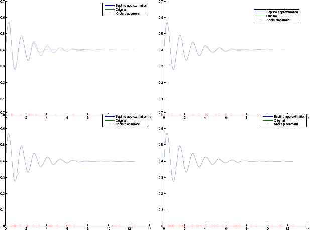
To test the behavior of the presented methodology for the optimization of knots placement of the B-spline basis in this case, all the procedure have been also adapted to this one-dimensional case. Not a large number of knots have been necessary to obtain sufficiently good results, as you can see in the corresponding figures.
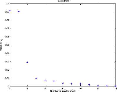
We can also see clearly, in the right column of Figure 1, how the evolution of the knots’ distribution tends to be located in the region where the function f1(x) change the most within its domain. The left column also shows the results of the approximating function, compared with the original one, using this B-spline function approximation. The corresponding Pareto front, taking also into account one of the errors in the approximations vs. the number of knots used, is shown in Figure 2.
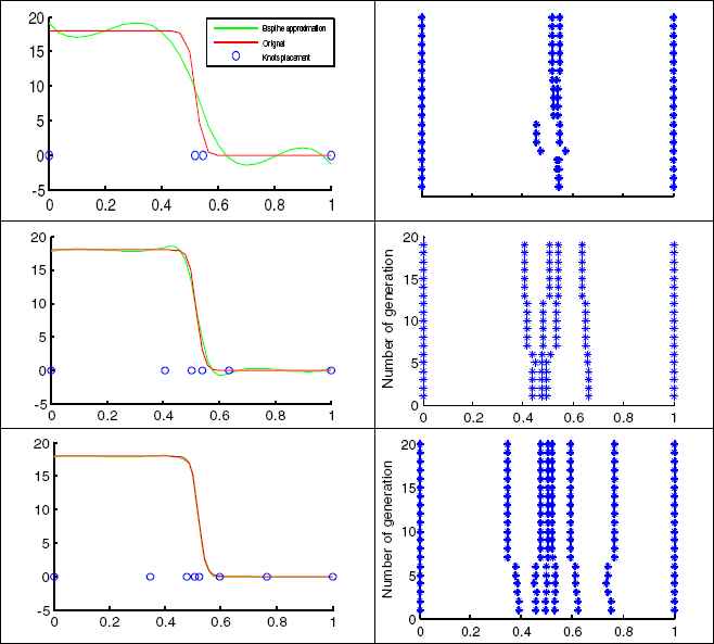
Approximating spline vs. actual function f1(x) (left) at final generation and distribution of knots in each generation (right) for 2, 4 and 6 interior knots respectively
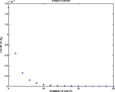
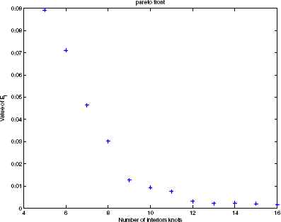
Pareto front of El error vs. number of knots for f1(x).
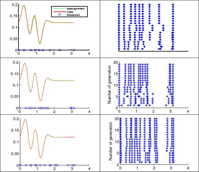
Approximating spline vs. actual function f2(x) (left) at final generation and distribution of knots in each generation (right) for 8, 11 and 14 interior knots respectively
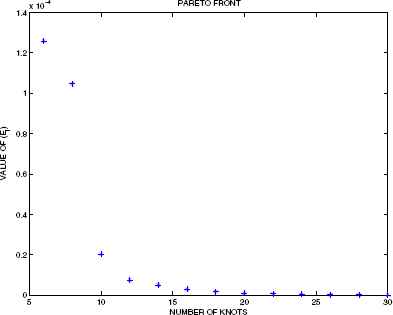
Pareto front of El error vs. number of knots for f2(x).
We can view clearly in all these cases that our results are quite better than the corresponding results included in the specified articles, with less interior knots; and always obtaining lower errors when using the same number of them or less number of generations.
Now we show in Figure 5 our results (with discrete errors of orders of 10−4 and 10−5 in any case) for the Example 3, also used as test example in 15.
Approximating splines vs. actual function f3(x) at final generation for 10, 15, 20 and 30 interior knots (marked on the x-axis) respectively.
And finally, in Figure 6 some graphical and numerical result for the Example 4, also considered in a classical paper 9 about this subject.
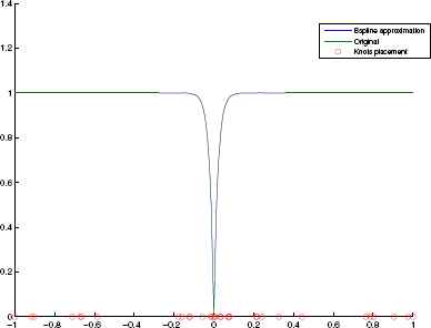
Graphical results for f4(x) with 29 interior knots (marked on the x-axis) and a discretized error of order 10−4
5.2. Examples of functions of two independent variables
We begin with a quite simple example of a paraboloid of revolution in the following example
Example 5:
F5 : [0, 1] × [0, 1] → ℝ
In order to analyze the behavior of the B-spline approximation in these cases, not too many knots will be used (just 10 to 20 knots in each variable interval). In Figure 7 it can be seen some particular results of the approximation of function F5(x, y) using bi-cubic smoothing variational splines.
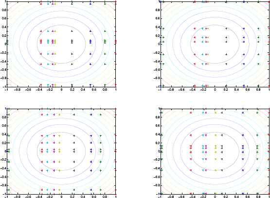
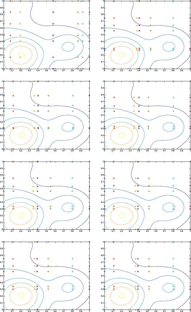
From top to down and left to right, evolution of the knots distribution every 5 generations for the function F5 (x, y).
Similar results can be obtained for a more complicated Example 6, where the well-known Franke’s function is considered. Graphics in Figure 9 show the results of the approximation with Bi-cubic smoothing variational splines in this case.
6. Conclusions
In this paper, a novel evolutionary MOGA methodology is presented for knots placement in the problem of cubic spline approximation of functions of one or two variables, showing the effectiveness of the strategy for different types of functions.
So, the goal of using a MOGA for placement of the knots in such cases of approximating functions by cubic or bi-cubic splines, of one or two variables, respectively, can be summarized as follows:
Example 6:
F6 : [0, 1] × [0, 1] → ℝ
Figures 8 and 10 represent the Pareto fronts for the application of this MOGA procedure to these last two examples. It is clear that the errors with the MOGA tends to be reduced when the number of knots to construct the smoothing B-spline basis increases, but also increases (significantly in this case) the corresponding computational effort.
- (1)
It has been sufficiently proven that the placement of the knots in spline approximation has an important and considerable effect on the behavior of the final results, but the optimal placement or location of knots is not known a priori;
- (2)
The number of knots to be used in classical approaches, should be selected a priori by the designer; but using MOGA, a Pareto front for different or variable number of knots used can also be directly optimized.
Pareto front of El error vs. number of knots for F4(x).
From top to down and left to right, evolution of the knots distribution every 5 generations for the function F6 (x, y).
Pareto front of El error vs. number of knots for F6(x).
Many simulations have been carried out, showing that increasing the number of knots in the definition of the cubic, or bi-cubic B-splines, also increases the accuracy of the approximation, but only up to a certain limit, where the corresponding computation effort is not worth enough comparing with the small possible reduction in the corresponding errors. So we can affirm without any doubt, that this proposed procedure have much better performance and results than such as the selected knots within an equally spaced distribution of them, and many other classical approaches.
References
Cite this article
TY  - JOUR
AU  - P. González
AU  - H. Idais
AU  - M. Pasadas
AU  - M. Yasin
PY  - 2018
DA  - 2018/07/26
TI  - Evolutionary computation for optimal knots allocation in smoothing splines of one or two variables
JO  - International Journal of Computational Intelligence Systems
SP  - 1294
EP  - 1306
VL  - 11
IS  - 1
SN  - 1875-6883
UR  - https://doi.org/10.2991/ijcis.11.1.96
DO  - 10.2991/ijcis.11.1.96
ID  - González2018
ER  -